Lesson 5. The Fastest Way to Process Rasters in R
Learning Objectives
After completing this tutorial, you will be able to:
- Calculate NDVI using NAIP multispectral imagery in
R. - Describe what a vegetation index is and how it is used with spectral remote sensing data.
What You Need
You will need a computer with internet access to complete this lesson and the data for week 7 of the course.
Below you will find several benchmark tests that demonstrate the fastest way to process raster data in R.
The summary:
- For basic raster math - for example subtracting two rasters, it’s fastest to just perform the math!
- For more complex math calculations like NDVI, the overlay function is faster.
- Raster bricks are always faster!
# load spatial packages
library(raster)
library(rgdal)
library(rgeos)
# turn off factors
options(stringsAsFactors = FALSE)
# import the naip pre-fire data
naip_multispectral_st <- stack("data/week-07/naip/m_3910505_nw_13_1_20130926/crop/m_3910505_nw_13_1_20130926_crop.tif")
# create a function that subtracts two rasters

diff_rasters <- function(b1, b2){
  # this function calculates the difference between two rasters of the same CRS and extent
  # input: 2 raster layers of the same extent, crs that can be subtracted
  # output: a single different raster of the same extent, crs of the input rasters
  diff <- b2 - b1
  return(diff)
}
Let’s use the same function on some more useful data. Calculate the difference between the lidar DSM and DEM using this function.
# import lidar rasters
lidar_dsm <- raster(x = "data/week-03/BLDR_LeeHill/pre-flood/lidar/pre_DSM.tif")
lidar_dtm <- raster(x = "data/week-03/BLDR_LeeHill/pre-flood/lidar/pre_DTM.tif")

# calculate difference  - make sure you provide the rasters in the right order!
lidar_chm <- overlay(lidar_dtm, lidar_dsm,
                     fun = diff_rasters)

plot(lidar_chm,
     main = "Canopy Height Model derived using the overlay function \n and the band_diff function\n that you created")

library(microbenchmark)
# is it faster?
microbenchmark((lidar_dsm - lidar_dsm), times = 10)
## Unit: seconds
##                     expr      min      lq     mean   median       uq
##  (lidar_dsm - lidar_dsm) 1.086393 1.12504 1.140462 1.132166 1.148794
##       max neval
##  1.229389    10

microbenchmark(overlay(lidar_dtm, lidar_dsm,
                     fun = diff_rasters), times = 10)
## Unit: seconds
##                                               expr    min       lq
##  overlay(lidar_dtm, lidar_dsm, fun = diff_rasters) 1.7922 1.809741
##      mean   median       uq      max neval
##  1.824008 1.827214 1.830336 1.855017    10
The overlay function is actually not faster when you are performing basic raster calculations in R. However, it does become faster when using rasterbricks and more complex calculations.
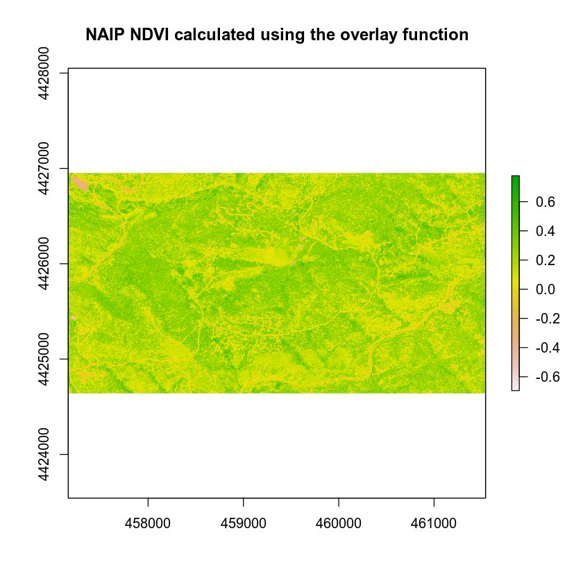
Let’s test things out on NDVI which is a more complex equation.
# calculate ndvi using the overlay function
# you will have to create the function on your own!
naip_ndvi_ov <- overlay(naip_multispectral_st[[1]],
        naip_multispectral_st[[4]],
        fun = normalized_diff)

plot(naip_ndvi_ov,
     main = "NAIP NDVI calculated using the overlay function")

Don’t believe overlay is faster? Let’s test it using a benchmark.
library(microbenchmark)
# is the raster in memory?
inMemory(naip_multispectral_st)
## [1] FALSE

# How long does it take to calculate ndvi without overlay.
microbenchmark((naip_multispectral_st[[4]] - naip_multispectral_st[[1]]) / (naip_multispectral_st[[4]] + naip_multispectral_st[[1]]), times = 5)
## Unit: seconds
##                                                                                                                      expr
##  (naip_multispectral_st[[4]] - naip_multispectral_st[[1]])/(naip_multispectral_st[[4]] +      naip_multispectral_st[[1]])
##       min       lq     mean   median       uq      max neval
##  2.528051 2.560168 2.583259 2.566227 2.614948 2.646902     5


# is overlay faster?
microbenchmark(overlay(naip_multispectral_st[[1]],
        naip_multispectral_st[[4]],
        fun = normalized_diff), times = 5)
## Unit: seconds
##                                                                                         expr
##  overlay(naip_multispectral_st[[1]], naip_multispectral_st[[4]],      fun = normalized_diff)
##       min       lq     mean   median       uq      max neval
##  1.844418 1.867522 1.868953 1.868801 1.879466 1.884559     5

# what if you make your stack a brick - is it faster?
naip_multispectral_br <- brick(naip_multispectral_st)
inMemory(naip_multispectral_br)
## [1] FALSE

microbenchmark(overlay(naip_multispectral_br[[1]],
        naip_multispectral_br[[4]],
        fun = normalized_diff), times = 5)
## Unit: seconds
##                                                                                         expr
##  overlay(naip_multispectral_br[[1]], naip_multispectral_br[[4]],      fun = normalized_diff)
##       min       lq     mean   median       uq      max neval
##  1.451341 1.633023 1.683456 1.695315 1.696663 1.940938     5
Notice that the results above suggest that the overlay() function is in fact just a bit faster than the regular raster math approach. This may seem minor now. However, you are only working with 55mb files. This will save processing time in the long run, as you work with larger raster files.
Share on
Twitter Facebook Google+ LinkedIn
Leave a Comment