Lesson 6. Landsat Remote Sensing tif Files in R
Learning Objectives
After completing this tutorial, you will be able to:
- Use
list.files()to create a subsetted list of file names within a specified directory on your computer. - Create a raster stack from a list of
.tiffiles inR. - Plot various band combinations using a rasterstack in
RwithplotRGB().
What You Need
You will need a computer with internet access to complete this lesson and the data for week 7 of the course.
In the previous lesson, you learned how to import a multi-band image into R using
the stack() function. You then plotted the data as a composite, RGB (and CIR) image
using plotRGB(). However, sometimes data are downloaded in individual bands rather
than a composite raster stack.
In this lesson you will learn how to work with Landsat data in R. In this case, your
data are downloaded in .tif format with each .tif file representing a single
band rather than a stack of bands.
About Landsat Data
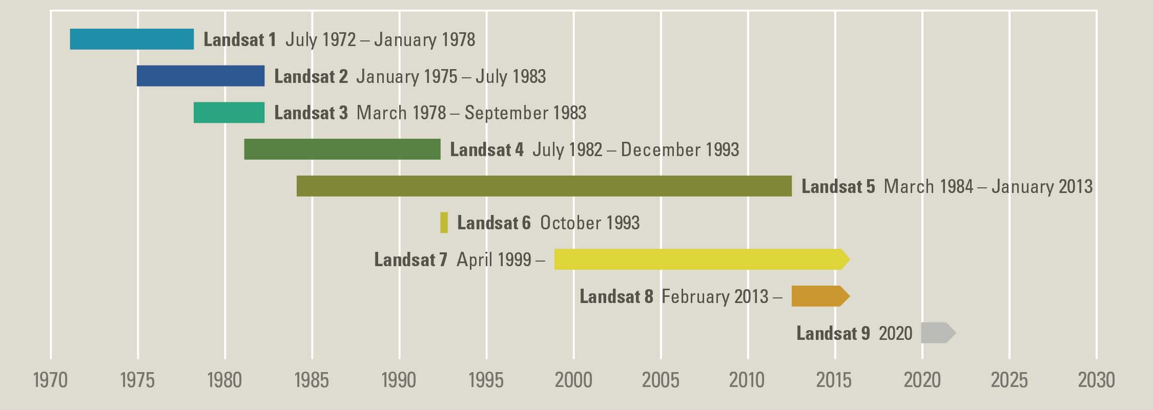
At over 40 years, the Landsat series of satellites provides the longest temporal record of moderate resolution multispectral data of the Earth’s surface on a global basis. The Landsat record has remained remarkably unbroken, proving a unique resource to assist a broad range of specialists in managing the world’s food, water, forests, and other natural resources for a growing world population. It is a record unmatched in quality, detail, coverage, and value. Source: USGS
Landsat data is a multispectral dataset collected from space. The multispectral bands and associated spatial resolution of the first 9 bands in the Landsat 8 sensor are listed below.
Landsat 8 Bands
| Band | Wavelength range (nanometers) | Spatial Resolution (m) | Spectral Width (nm) |
|---|---|---|---|
| Band 1 - Coastal aerosol | 430 - 450 | 30 | 2.0 |
| Band 2 - Blue | 450 - 510 | 30 | 6.0 |
| Band 3 - Green | 530 - 590 | 30 | 6.0 |
| Band 4 - Red | 640 - 670 | 30 | 0.03 |
| Band 5 - Near Infrared (NIR) | 850 - 880 | 30 | 3.0 |
| Band 6 - SWIR 1 | 1570 - 1650 | 30 | 8.0 |
| Band 7 - SWIR 2 | 2110 - 2290 | 30 | 18 |
| Band 8 - Panchromatic | 500 - 680 | 15 | 18 |
| Band 9 - Cirrus | 1360 - 1380 | 30 | 2.0 |
Get to Know Landsat 8 Filenames
When working with Landsat, it is important to understand both the metadata and the file naming convention. The metadata tell you how the data were processed, where the data are from and how they are structured.
The file names, tell you what sensor collected the data, the date the data were collected, and more.
Landsat file naming convention
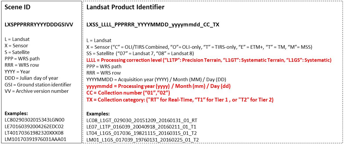
Let’s have a look at one of the files and use the image above to guide us through understanding the file name.
File: LC80340322016205LGN00_sr_band1_crop.tif
| Sensor | Sensor | Satellite | WRS path | WRS row | ||||
|---|---|---|---|---|---|---|---|---|
| L | C | 8 | 034 | 032 | 2016 | 205 | LGN | 00 |
| Landsat | OLI & TIRS | Landsat 8 | path = 034 | row = 032 | year = 2016 | Julian day= 205 | Ground station: LGN | Archive (first version): 00 |
- L: Landsat
- X: Sensor
- C = OLI & TIRS O = OLI only T = IRS only E = ETM+ T = TM M = MSS
- S Satelite
- PPP
- RRR
- YYYY = Year
- DDD = Julian DAY of the year
- GSI - Ground station ID
- VV = Archive Version
More here breaking down the file name.
Julian Day
In class, we won’t spend a lot of time on Julian days. For the purpose of working with Landsat and MODIS data, what you need to know is that the calendar year Julian day represents the numeric day of the year. So Jan 1 = day 1. Feb 1 = day 32. And so on.
There are several links at the bottom of this page that provide tables that help you convert Julian days to actual date.
Landsat tif Files in R
Next, you can open the Landsat data in R.
# load spatial packages
library(raster)
library(rgdal)
library(rgeos)

# turn off factors
options(stringsAsFactors = FALSE)
If you look at the Landsat directory for the week_07 data, you will see that each of the individual bands is stored individually as a GeoTIFF rather than being stored as a stacked or layered, multi-band raster.
Why would they store the data this way?
Conventionally Landsat was stored in a file format called HDF - hierarchical data format. However that format, while extremely efficient, is a bit more challenging to work with. In recent years USGS has started to make each band of a Landsat scene available as a .tif file. This makes it a bit easier to use across many different programs and platforms.
You have already been working with the geotiff file format in this class! You will thus use many of the same functions you used previously, to work with Landsat.
Get List of Files
To begin, let’s explore your file directory in R, You can use list.files() to
grab a list of all files within any directory on your computer.
# get list of all tifs
list.files("data/week-07/landsat/LC80340322016205-SC20170127160728/crop")
##  [1] "LC80340322016205LGN00_bqa_crop.tif"
##  [2] "LC80340322016205LGN00_cfmask_conf_crop.tif"
##  [3] "LC80340322016205LGN00_cfmask_crop.tif"
##  [4] "LC80340322016205LGN00_sr_band1_crop.tif"
##  [5] "LC80340322016205LGN00_sr_band2_crop.tif"
##  [6] "LC80340322016205LGN00_sr_band3_crop.tif"
##  [7] "LC80340322016205LGN00_sr_band4_crop.tif"
##  [8] "LC80340322016205LGN00_sr_band5_crop.tif"
##  [9] "LC80340322016205LGN00_sr_band6_crop.tif"
## [10] "LC80340322016205LGN00_sr_band7_crop.tif"
## [11] "LC80340322016205LGN00_sr_cloud_crop.tif"
## [12] "LC80340322016205LGN00_sr_ipflag_crop.tif"
You can also use list.files() with the pattern argument. This allows you to specify
a particular pattern that further subsets your data. In this case, you just want
to look at a list of files with the extension: .tif. Note that it is important
that the file ends with .tif. So you use the dollar sign at the end of your
pattern to tell R to only grab files that end with .tif.
pattern = ".tif$"
# but really you just want the tif files
all_landsat_bands <- list.files("data/week-07/landsat/LC80340322016205-SC20170127160728/crop",
                      pattern = ".tif$",
                      full.names = TRUE) # make sure you have the full path to the file
all_landsat_bands
##  [1] "data/week-07/landsat/LC80340322016205-SC20170127160728/crop/LC80340322016205LGN00_bqa_crop.tif"
##  [2] "data/week-07/landsat/LC80340322016205-SC20170127160728/crop/LC80340322016205LGN00_cfmask_conf_crop.tif"
##  [3] "data/week-07/landsat/LC80340322016205-SC20170127160728/crop/LC80340322016205LGN00_cfmask_crop.tif"
##  [4] "data/week-07/landsat/LC80340322016205-SC20170127160728/crop/LC80340322016205LGN00_sr_band1_crop.tif"
##  [5] "data/week-07/landsat/LC80340322016205-SC20170127160728/crop/LC80340322016205LGN00_sr_band2_crop.tif"
##  [6] "data/week-07/landsat/LC80340322016205-SC20170127160728/crop/LC80340322016205LGN00_sr_band3_crop.tif"
##  [7] "data/week-07/landsat/LC80340322016205-SC20170127160728/crop/LC80340322016205LGN00_sr_band4_crop.tif"
##  [8] "data/week-07/landsat/LC80340322016205-SC20170127160728/crop/LC80340322016205LGN00_sr_band5_crop.tif"
##  [9] "data/week-07/landsat/LC80340322016205-SC20170127160728/crop/LC80340322016205LGN00_sr_band6_crop.tif"
## [10] "data/week-07/landsat/LC80340322016205-SC20170127160728/crop/LC80340322016205LGN00_sr_band7_crop.tif"
## [11] "data/week-07/landsat/LC80340322016205-SC20170127160728/crop/LC80340322016205LGN00_sr_cloud_crop.tif"
## [12] "data/week-07/landsat/LC80340322016205-SC20170127160728/crop/LC80340322016205LGN00_sr_ipflag_crop.tif"
Above, you use the $ after .tif to tell R to look for files that end with .tif.
This is a good start but there is one more condition that we’d like to meet. We
only want the .tif files that are spectral bands. Notice that some of your files
have text that includes “mask”, flags, etc. Those are all additional layers that
you don’t need right now. You just need the spectral data saved in bands 1_7.
Mini Introduction to Regular Expressions
Thus, you want to grab all bands that both end with .tif AND contain the text
“band” in them. To do this you use the function glob2rx() which allows you to specify
both conditions using what is called regular expressions.
A regular expression is a sequence of characters that defines a search pattern. Here
you tell R to select all files that have the word band
in the filename. You use a * sign before and after band because you don’t know
exactly what text will occur before or after band. You use .tif$ to tell R that
each file needs to end with .tif.
all_landsat_bands <- list.files("data/week-07/landsat/LC80340322016205-SC20170127160728/crop",
           pattern = glob2rx("*band*.tif$"),
           full.names = TRUE) # use the dollar sign at the end to get all files that END WITH
all_landsat_bands
## [1] "data/week-07/landsat/LC80340322016205-SC20170127160728/crop/LC80340322016205LGN00_sr_band1_crop.tif"
## [2] "data/week-07/landsat/LC80340322016205-SC20170127160728/crop/LC80340322016205LGN00_sr_band2_crop.tif"
## [3] "data/week-07/landsat/LC80340322016205-SC20170127160728/crop/LC80340322016205LGN00_sr_band3_crop.tif"
## [4] "data/week-07/landsat/LC80340322016205-SC20170127160728/crop/LC80340322016205LGN00_sr_band4_crop.tif"
## [5] "data/week-07/landsat/LC80340322016205-SC20170127160728/crop/LC80340322016205LGN00_sr_band5_crop.tif"
## [6] "data/week-07/landsat/LC80340322016205-SC20170127160728/crop/LC80340322016205LGN00_sr_band6_crop.tif"
## [7] "data/week-07/landsat/LC80340322016205-SC20170127160728/crop/LC80340322016205LGN00_sr_band7_crop.tif"
Open the .tif Files in R
Now you have a list of all of the Landsat bands in your folder. You could chose to
open each file individually using the raster() function.
# get first file
all_landsat_bands[2]
## [1] "data/week-07/landsat/LC80340322016205-SC20170127160728/crop/LC80340322016205LGN00_sr_band2_crop.tif"
landsat_band2 <- raster(all_landsat_bands[2])
plot(landsat_band2,
     main = "Landsat cropped band 2\nCold Springs fire scar",
     col = gray(0:100 / 100))

However, that is not a very efficient approach.
It’s more efficiently to open all of the layers together as a stack. Then you can
access each of the bands and plot / use them as you want. You can do that using the
stack() function.
# stack the data
landsat_stack_csf <- stack(all_landsat_bands)
# then turn it into a brick
landsat_csf_br <- brick(landsat_stack_csf)
# view stack attributes
landsat_csf_br
## class      : RasterBrick
## dimensions : 177, 246, 43542, 7  (nrow, ncol, ncell, nlayers)
## resolution : 30, 30  (x, y)
## extent     : 455655, 463035, 4423155, 4428465  (xmin, xmax, ymin, ymax)
## crs        : +proj=utm +zone=13 +datum=WGS84 +units=m +no_defs +ellps=WGS84 +towgs84=0,0,0
## source     : memory
## names      : LC8034032//band1_crop, LC8034032//band2_crop, LC8034032//band3_crop, LC8034032//band4_crop, LC8034032//band5_crop, LC8034032//band6_crop, LC8034032//band7_crop
## min values :                     0,                     0,                     0,                     0,                     0,                     0,                     0
## max values :                  3488,                  3843,                  4746,                  5152,                  5674,                  4346,                  3767
Let’s plot each individual band in your brick.
plot(landsat_csf_br,
     col = gray(20:100 / 100))

# get list of each layer name
names(landsat_csf_br)
## [1] "LC80340322016205LGN00_sr_band1_crop"
## [2] "LC80340322016205LGN00_sr_band2_crop"
## [3] "LC80340322016205LGN00_sr_band3_crop"
## [4] "LC80340322016205LGN00_sr_band4_crop"
## [5] "LC80340322016205LGN00_sr_band5_crop"
## [6] "LC80340322016205LGN00_sr_band6_crop"
## [7] "LC80340322016205LGN00_sr_band7_crop"

# remove the filename from each band name for pretty plotting
names(landsat_csf_br) <- gsub(pattern = "LC80340322016205LGN00_sr_", replacement = "", names(landsat_csf_br))
plot(landsat_csf_br,
     col = gray(20:100 / 100))

Plot RGB Composite Band Images with Landsat in R
Next, let’s plot an RGB image using Landsat. Refer to the Landsat bands in the table at the top of this page to figure out the red, green and blue bands. Or read the ESRI Landsat 8 band combinations post.
par(col.axis = "white", col.lab = "white", tck = 0)
plotRGB(landsat_csf_br,
     r = 4, g = 3, b = 2,
     stretch = "lin",
     axes = TRUE,
     main = "RGB composite image\n Landsat Bands 4, 3, 2")
box(col = "white")

Now we’ve created a red, green blue color composite image. Remember this is what your eye would see. What happens if you plot the near infrared band instead of red? Try the following combination:
par(col.axis = "white", col.lab = "white", tck = 0)
plotRGB(landsat_csf_br,
     r = 5, g = 4, b = 3,
     stretch = "lin",
     axes = TRUE,
     main = "Color infrared composite image\n Landsat Bands 5, 4, 3\n Post Fire Data")
box(col = "white")

Optional Challenge
Using the ESRI Landsat 8 band combinations post as a guide. Plot the following Landsat band combinations:
- False color
- Color infrared
- Agriculture
- Healthy vegetation
Be sure to add a title to each of your plots that specifies the band combination.
Additional Resources
Share on
Twitter Facebook Google+ LinkedIn
Leave a Comment