Document Your Science Using R Markdown and R
Welcome to Week One!
Welcome to week 1 of Earth Analytics! In week 1 you will explore data
related to the 2013 Colorado Floods. In your homework, you will get
R and RStudio set up on your laptop and learn how to create an R Markdown
document and convert it to a pdf using knitr. Finally you will create a short
report after reading articles on the 2013 Colorado Floods.
Homework Week 1
Due: Friday 8 September 2017 by 8PM Mountain Time
1. Readings
Open Science Readings
Read the open science related articles below.
- The value of open science
- Five selfish reasons to work reproducibly - Florian Markowetz
- Computing Workflows for Biologists: A Roadmap
View Slideshow: Share, Publish & Archive Code & Data
Flood Readings
Read the following articles and listen to the 7 minute interview with Suzanne Anderson (faculty here at CU Boulder).
-
Read the short article and listen to the 7 minute interview with Suzanne Anderson: To listen - click on the “ Listen” icon on the page Study: 2013 Front Range floods caused a thousand year’s worth of erosion
2. Watch Flood Video
Watch this video to learn more about the 2013 Colorado floods and some of the data that can be used to better understand the drivers and impacts of those floods.
Before and After Google Earth Fly Through
3. Review Lessons
After you’ve read the readings and watched the videos, complete the homework
assignment below. Review the Set Up R lessons. (see links
on the left hand side of this page).
Following the lessons, setup R, RStudio and a
working directory that will contain the data you will use for the entire course.
IMPORTANT: if you working directory is not setup right - you won’t be able to
follow along in class. Also you won’t be able to test your code when you submit assignments
to give you partial credit!
Once everything is setup, review the second set of lessons (R Markdown intro) which walk you
through creating R Markdown documents and knitting them to .html format. If you
already know rmarkdown, be sure to review the lessons anyway - particularly
the ones about file organization and why you use this workflow in science.
Important: Review ALL of the lessons and have your computer setup BEFORE class begins next week. You will be behind if these things are not setup / complete before week 2.
4. Complete Assignment Below
After you have reviewed the lessons above, complete the assignment below.
Submit your .html document and R Markdown document to the D2L course drop box
by Friday 8 September 2017 by 8PM Mountain Time.
Homework Submission: Create A Report Using Knitr & RMarkdown
1. Create R Markdown file
- Create a new rmarkdown
.Rmdfile inRstudio. Name the file:yourLastName-firstInitial-week01.Rmdexample:wasser-l-week01.Rmd- Save your
.Rmdfile in the ``\earth-analytics` working directory that you created for this class using the lessons. IMPORTANT: do not save the.Rmdfile in the\datadirectory. Your code won’t run! - Add an
author:line to theYAMLheader at the top of your.Rmddocument. - Make sure the YAML has a
date:element. - Add a
title:that represents the contents of your report. Example:2013 Colorado floods - earth analytics fall 2017
- Save your
2. Write Up the Following
At the top of the R Markdown document (BELOW THE YAML HEADER), writeup the following (Use the readings and video assigned above to answer these questions):
- Write a 1 page overview of the events that lead to the flooding that occurred in 2013. In this writeup, be sure to explain how the floods impacts people in Colorado. NOTE: this text will be used in the final report that you create about the 2013 floods so the better this text is now, the less you will have to do later! Read the articles and craft this write up carefully. Be sure to cite at least 3 of the articles above (or others that you find) in your write up.
- At the bottom of your report, write 1-2 paragraphs that describe:
- What open science is and why it is important
- How approaches including using
R Markdowncan be helpful to both you and your colleagues that you work with on a project and to following open science principles in general.
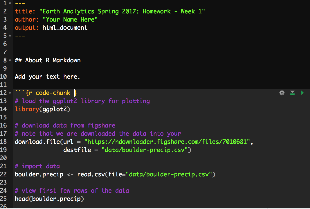
3. Add Code to Your Document
- Create a new CODE CHUNK.
- Copy and paste the code BELOW into the code chunk that you just created.
- Below the code chunk in your
R Markdowndocument, add some TEXT that describes what the plot that you created shows - interpret what you see in the data.
BONUS: If you know R, clean up the plot by adding labels and a title. Or better
yet, use ggplot2!
# load the ggplot2 library for plotting
library(ggplot2)

# download data from figshare
# note that you are downloading the data into your data directory
download.file(url = "https://ndownloader.figshare.com/files/7010681",
              destfile = "data/boulder-precip.csv",
              method = "libcurl")

# if the code above doesn't allow you to download the data, remove the method =
# "libcurl" argument! Also note that you may get a warning that you are not able to
# download the data twice. That is ok!

# import data
boulder_precip <- read.csv(file="data/boulder-precip.csv")

# view first few rows of the data
head(boulder_precip)
##     X       DATE PRECIP
## 1 756 2013-08-21    0.1
## 2 757 2013-08-26    0.1
## 3 758 2013-08-27    0.1
## 4 759 2013-09-01    0.0
## 5 760 2013-09-09    0.1
## 6 761 2013-09-10    1.0

# when you download the data you create a `data.frame`
# view each column of the data frame using it's name (or header)
boulder_precip$DATE
##  [1] "2013-08-21" "2013-08-26" "2013-08-27" "2013-09-01" "2013-09-09"
##  [6] "2013-09-10" "2013-09-11" "2013-09-12" "2013-09-13" "2013-09-15"
## [11] "2013-09-16" "2013-09-22" "2013-09-23" "2013-09-27" "2013-09-28"
## [16] "2013-10-01" "2013-10-04" "2013-10-11"

# view the precip column
boulder_precip$PRECIP
##  [1] 0.1 0.1 0.1 0.0 0.1 1.0 2.3 9.8 1.9 1.4 0.4 0.1 0.3 0.3 0.1 0.0 0.9
## [18] 0.1

# qplot stands for quick plot. It is a function in the ggplot2 library.
# Let's use it to plot our data
qplot(x = boulder_precip$DATE,
      y = boulder_precip$PRECIP)

If your code ran properly, the plot output should look like the image above.
Troubleshooting: Missing Plot
If the code above did not produce a plot, please check the following:
Check Your Working Directory
If the path to your file is not correct, then the data won’t load into R.
If the data don’t load into R, then you can’t work with it or plot it.
To figure out your current working directory use the command: getwd()
Next, go to your finder or file explorer on your computer. Navigate to the path
that R gives you when you type getwd() in the console. It will look something
like the path example: /Users/your-username/documents/earth-analytics
# check your working directory
getwd()

## [1] "/Users/lewa8222/documents/earth-analytics"
In the example above, note that my USER directory is called lewa8222. Yours
is called something different. Is there a data directory within the earth-analytics
directory?
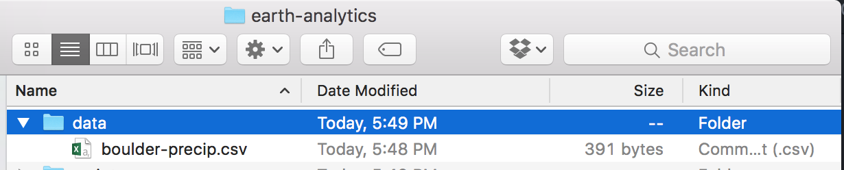
If not, review the working directory lesson
to ensure your working directory is SETUP properly on your computer and in RStudio.
Class Participation - Flood Diagram Activity
While attendance is not explicitly tracked, participation in this course counts towards your grade. This week, please be sure that your name is associated with one of the diagrams posted in the piazza forum. In class you worked in groups so it is ok if multiple people are associated with one diagram. Just be sure your name is there so you get credit and if it isn’t - please edit your post and add your names above the image!
Grade Rubric
Your assignment will be graded using the rubric below. Remember as always - NO LATE ASSIGNMENTS will be accepted. Please do not ask. Submit what you have done - as is - ON TIME!
R Markdown Report Syntax & Code (20%)
| Full credit | No credit | ||
|---|---|---|---|
| HTML and RMD submitted | |||
| YAML contains title, author and date | |||
| File is named with last name-first initial week 1 | |||
| Grammar and spelling is excellent - no misspellings |
R Markdown Report Code Runs (20%)
| Full credit | No credit | |
|---|---|---|
| Code chunk contains code and runs (a correct plot is produced) | ||
| Code chunk is formatted correctly |
R Markdown Report Writeup (60%)
| Full credit | No credit | |
|---|---|---|
| 1 page overview of the flood is thoughtful, accurately describes the flood events and location and clearly references readings | ||
| Flood report identifies the drivers and impacts of the flood | ||
| Flood report discusses the elements that triggered the 2013 colorado floods | ||
| Open science writeup references readings | ||
| Open science writeup defines open science correctly and documents its importance following the readings |
Share on
Twitter Facebook Google+ LinkedIn