About Landsat Scenes

Landsat satellites orbit the earth continuously collecting images of the Earth’s surface. These images, are divided into smaller regions - known as scenes.

Landsat images are usually divided into scenes for easy downloading. Each Landsat scene is about 115 miles long and 115 miles wide (or 100 nautical miles long and 100 nautical miles wide, or 185 kilometers long and 185 kilometers wide). -wikipedia

Challenges Working with Landsat Remote Sensing Data

In the previous lessons, you learned how to import a set of geotiffs that made up the bands of a landsat raster. Each geotiff file was a part of a Landsat scene, that had been downloaded for this class by your instructor. The scene was further cropped to reduce the file size for the class.

You ran into some challenges when you began to work with the data. The biggest problem was a large cloud and associated shadow that covered your study area of interest - the Cold Springs fire burn scar.

Dealing with Clouds & Shadows in Remote Sensing Data

Clouds and atmospheric conditions present a significant challenge when working with multispectral remote sensing data. Extreme cloud cover and shadows can make the data in those areas, un-usable given reflectance values are either washed out (too bright - as the clouds scatter all light back to the sensor) or are too dark (shadows which represent blocked or absorbed light).

In this lesson you will learn how to deal with clouds in your remote sensing data. There is no perfect solution of course. You will just learn one approach.

Begin by loading your spatial libraries.

# import spatial packages
library(raster)
library(rgdal)
library(rgeos)
# turn off factors
options(stringsAsFactors = FALSE)

Next, you will load the landsat bands that you loaded previously in your homework.

# create a list of all landsat files that have the extension .tif and contain the word band.
all_landsat_bands <- list.files("data/week-08/landsat/LC80340322016189-SC20170128091153/crop",
           pattern = glob2rx("*band*.tif$"),
           full.names = TRUE) # use the dollar sign at the end to get all files that END WITH
# create spatial raster stack from the list of file names
all_landsat_bands_st <- stack(all_landsat_bands)
all_landsat_bands_br <- brick(all_landsat_bands_st)

When you plotted the pre-fire image, you noticed a large cloud in your scene. Notice as i’m plotting below, i’m adding a few parameters to force R to add a title to my plot.

Data Tip: Check out the additional “How to” lessons for this week to learn more about creating nicer plots in R.

# turn the axis color to white and turn off ticks
par(col.axis = "white", col.lab = "white", tck = 0)
# plot the data - be sure to turn AXES to T (you just color them white)
plotRGB(all_landsat_bands_br,
        r = 4, g = 3, b = 2,
        stretch = "hist",
        main = "Pre-fire RGB image with cloud\n Cold Springs Fire",
        axes = TRUE)
# turn the box to white so there is no border on your plot
box(col = "white")

Raster Masks

Often (but not always) remote sensing data come with mask layers. These layers identify pixels that are likely representative of a cloud or shadow that have been generated by whomever processed the data. When you download Landsat 8 data from Earth Explorer, the data came with 2 processed cloud mask raster layers.

1. LC80340322016189-SC20170128091153/crop/LC80340322016189LGN00_cfmask_crop.tif
2. LC80340322016189-SC20170128091153/crop/LC80340322016189LGN00_cfmask_conf_crop.tif

Let’s have a look at these layers next.

# open cloud mask layer
cloud_mask_189_conf <- raster("data/week-08/landsat/LC80340322016189-SC20170128091153/crop/LC80340322016189LGN00_cfmask_conf_crop.tif")
plot(cloud_mask_189_conf,
  main = "Landsat Julian Day 189 - Cloud mask layer.")

Next, you can plot the second mask layer. Do you notice any difference between the two?

# apply shadow mask
cloud_mask_189 <- raster("data/week-08/landsat/LC80340322016189-SC20170128091153/crop/LC80340322016189LGN00_cfmask_crop.tif")
plot(cloud_mask_189,
  main = "Landsat Julian Day 189 - Cloud mask layer with shadows.")

What Do the Metadata Tell Us?

You just explored two layers that potentially have information about cloud cover. However what do the values stored in those rasters mean? You can refer to the metadata provided when you downloaded the Landsat data to learn more about how each layer in your landsat dataset are both stored and calculated.

Let’s open the metadata file: data/week-08/landsat/LC80340322016189-SC20170128091153/LC80340322016189LGN00.xml What does it tell us?

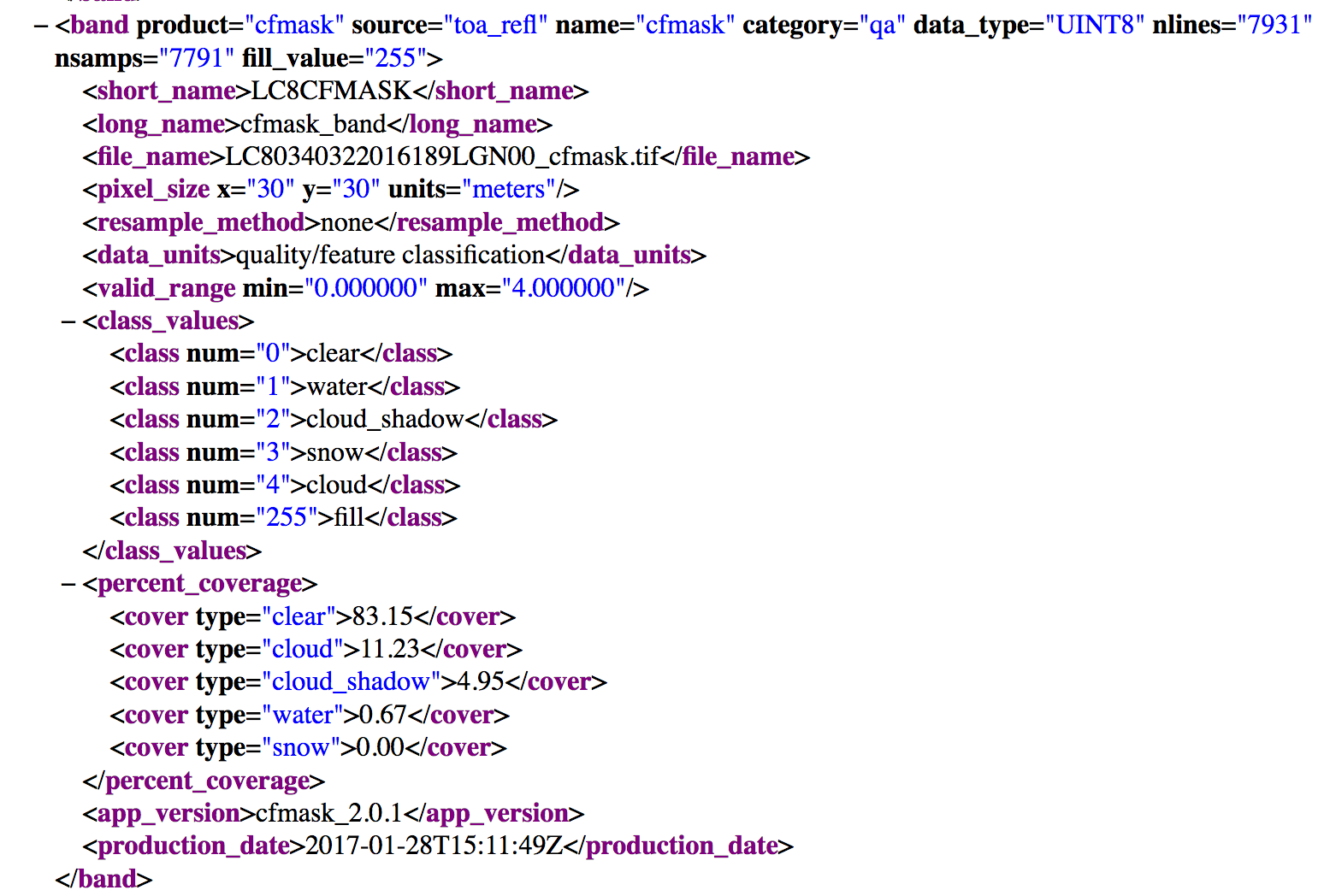
When you download remote sensing data, often (but not always), you will find layers that tell us more about the error and uncertainty in the data. Often whomever created the data will do some of the work for us to detect where clouds and shadows are - given they are common challenges that you need to work around when using remote sensing data.

In this case, if you study the metadata you can see that your cfmask.tif file contains several classes. 1, 2, and 4 represent clouds and shadows. These might be values of pixels that you want to mask from your analysis. More on this later.

Cloud Masks in R

You can use the cloud mask layer to identify pixels that are likely to be clouds or shadows. You can then set those pixel values to NA so they are not included in your quantitative analysis in R.

When you say “mask”, you are talking about a layer that “turns off” or sets to NA, the values of pixels in a raster that you don’t want to include in an analysis. It’s very similar to setting data points that equal -9999 to NA in a time series data set. You are just doing it with spatial raster data instead.

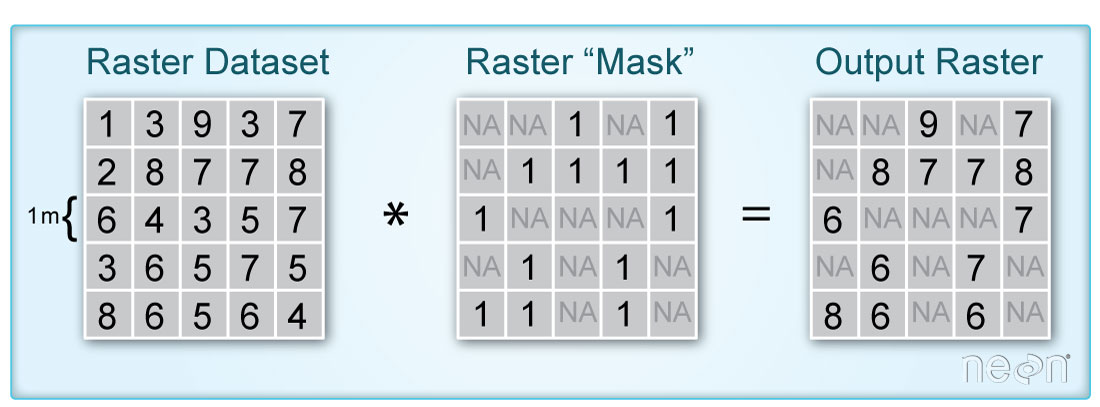
Create Mask Layer in R

To create the mask this you do the following:

1. You make sure you use a raster layer that is the SAME EXTENT and the same pixel resolution as your landsat scene. In this case you have a mask layer that is already the same spatial resolution and extent as your landsat scene.
2. You then set all of the values in that layer that are clouds and / or shadows to NA
3. Finally you use the mask() function to set all pixel locations that were flagged as clouds or shadows in your mask to NA in your raster or in this case rasterstack.

In this case, you want to set all values greater than 0 in the raster mask to NA.

par(xpd = FALSE, mar = c(0, 0, 1, 5))
# create cloud & cloud shadow mask
cloud_mask_189[cloud_mask_189 > 0] <- NA
# plot the masked data
plot(cloud_mask_189,
     main = "The Raster Mask",
     col = c("green"),
     legend = FALSE,
     axes = FALSE,
     box = FALSE)
# add legend to map
par(xpd = TRUE) # force legend to plot outside of the plot extent
legend(x = cloud_mask_189@extent@xmax, cloud_mask_189@extent@ymax,
       c("Not masked", "Masked"),
       fill = c("green", "white"),
       bty = "n")

Notice in the image above, all pixels that are green represent pixels that are OK or not masked. This means they weren’t flagged as potential clouds or shadows. All pixels that are WHITE are masked - these are areas of clouds and shadows.

Apply a Mask

You can apply a mask to all of the bands in your raster stack which is convenient! Let’s use the mask() function to mask your data.

# mask the stack
all_landsat_bands_mask <- mask(all_landsat_bands_br, mask = cloud_mask_189)

# check the memory situation
inMemory(all_landsat_bands_mask)
## [1] TRUE
class(all_landsat_bands_mask)
## [1] "RasterBrick"
## attr(,"package")
## [1] "raster"

Notice that once you perform a calculation on the raster, it is now in your computer’s memory.

# plot RGB image
# first turn all axes to the color white and turn off ticks
par(col.axis = "white", col.lab = "white", tck = 0)
# then plot the data
plotRGB(all_landsat_bands_mask,
        r = 4, g = 3, b = 2,
        main = "Landsat RGB Image \n Are the clouds gone?",
        axes = TRUE)
box(col = "white")

Notice above that I didn’t have to use the stretch function to force the data to plot in R. This is because the extremely bright pixels which represented clouds, are now removed from your data.

# plot RGB image
# first turn all axes to the color white and turn off ticks
par(col.axis = "white", col.lab = "white", tck = 0)
# then plot the data
plotRGB(all_landsat_bands_mask,
        r = 4, g = 3, b = 2,
        stretch = "lin",
        main = "Landsat RGB Image \n Are the clouds gone?",
        axes = TRUE)
box(col = "white")

Next, you can calculate a vegetation index.

A Cloud’s Covering Your Study Area - What’s Next?

Now that you have discovered a problem with your data that will impact quantitative analysis of the data, what do you do?

Well, there are several options, most of which you won’t discuss in this class. However, one option is that you could go find a better image. You happen to know that the conditions before the fire were rather stable in 2016. So what if you could find an image from say - June that doesn’t have clouds?

In the next lesson, you will learn to use the EarthExplorer website to download remote sensing data.