Intro to R & Work with Time Series Data
Welcome to Week 2!
Welcome to week 2 of Earth Analytics! In week 02 you will learn how to work with data in R and RStudio. We will also learn how to work with time series data. To work with time series data you need to know how to deal with date and time fields and missing data. It is also helpful to know how to subset the data by date.
The data that you use this week is collected by US Agency managed sensor networks. We will use the USGS stream gage network data and NOAA / National Weather Service precipitation data. All of the data you work with were collected in Boulder, Colorado around the time of the 2013 floods.
Read the assignment below carefully. Use the class and homework lessons to help you complete the assignment.
Class Schedule
| time | topic | speaker | ||
|---|---|---|---|---|
| 9:30 - 9:45 AM | Review RStudio / R Markdown / questions | Leah | ||
| 9:45 - 10:45 | R coding session - Intro to Scientific programming with R | Leah | ||
| 10:45 - 11:00 | Break | |||
| 11:00 - 12:20 | R coding session continued | Leah |
Homework Week 2
1. Download Data
Important - Data Organization
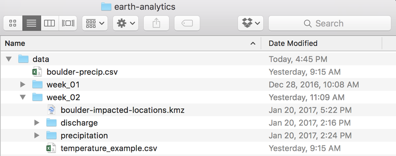
Before you begin this lesson, be sure that you’ve downloaded the dataset above. You will need to unzip the zip file. When you do this, be sure that your directory looks like the image below: note that all of the data are within the week_02 directory. The data are not nested within another directory. You may have to copy and paste your files into the correct directory to make this look right.
Why Data Organization Matters
It is important that your data are organized as specified in the lessons because:
- When the instructors grade your assignments, we will be able to run your code if your directory looks like the instructors’.
- It will be easier for you to follow along in class if your directory is the same as the instructors.
- It is good practice to learn how to organize your files in a way that makes it easier for your future self to find and work with your data!
2. Videos
Watch the following videos:
The Story of Lidar Data Video
How lidar works
3. Install QGIS & Review Homework Lessons
Install QGIS. Use the install QGIS homework lesson as a guide if needed. Then review all of the homework lessons - they will help you complete the submission below.
Homework (5 points): Due Friday Sept 15 @ 8pm
1. Create an R Markdown Document
Create a new R Markdown document. Name it: youLastName-yourFirstName-week02.rmd
2. Add the Text That You Wrote Last Week About the Flood Events
Add the text that you wrote for the first homework assignment to the top of your report. Then think about where in that text the plots below might fit best to better describe the events that occurred during the 2013 floods.
3. Add 4 Plots to Your R Markdown Document
Add the plots described below to your R Markdown file. IMPORTANT Please add a figure caption to each plot that describes the contents of the plot.
Add the code to produce the following 4 plots in your R Markdown document, using the homework lessons as a guide to walk you through. Use the pipes syntax that you learned in class to subset and summarize the data as required.
Use the data/week-02/precipitation/805325-precip-dailysum-2003-2013.csv file to create:
- PLOT 1: a plot of precipitation from 2003 to 2013 using the
ggplot()function. - PLOT 2: a plot that shows precipitation SUBSETTED from Aug 15 - Oct 15 2013 using the
ggplot()function.
Use the data/week-02/discharge/06730200-discharge-daily-1986-2013.csv file to create:
- PLOT 3: a plot of stream discharge from 1986 to 2013 using
ggplot()function. - PLOT 4: a plot that shows stream discharge SUBSETTED from Aug 15 - Oct 15 2013 using the
ggplot()function.
For all your plots be sure to do the following
Label Plots Appropriately
Be sure that each plot has:
- A figure caption that describes the contents of the plot.
- X and Y axis labels that include appropriate units.
- A carefully composed title that describes the contents of the plot.
Below each plot, describe and interpret what the plot shows. Describe how the data demonstrate an impact and / or a driver of the 2013 flood event.
Write Clean Code
Be sure that your code follows the style guidelines outlined in the write clean code lessons
Be sure to:
- Label each plot clearly. This includes a
title,xandyaxis labels. - Write clean code. This includes comments that document / describe the steps you take in your code and clean syntax following Hadley Wickham’s style guide.
- Convert date fields as appropriate.
- Clean no data values as appropriate.
- Show all of your code in the output
.htmlfile.
4. Graduate Students: Add a 5th Plot to Your .Rmd File
In addition to the plots above, add a plot of precipitation that spans from 1948 - 2013 using the 805333-precip-daily-1948-2013.csv file. For your plot be sure to:
- Subset the data temporally: Jan 1 2013 - Oct 15 2013.
- Summarize the data: plot DAILY total (sum) precipitation.
- Important: be sure to set the time zone as you are dealing with dates and times which are impacted by daylight saving time. Add:
tz = "America/Denver"to any statements involving time - but specifically to the line of code where you convert date / time to just a date!
Use the bonus lesson to guide you through creating this plot.
Bonus Points (For Grads and Undergrads)
Bonus Opportunity 1 (1 point): Generate and add to your report the plot of precipitation for 1948 - 2013 described above (required for all graduate students).
Then, receive a bonus point for:
- Identifying an anomaly or change in the data that you can clearly see when you plot it.
- Suggesting how to address that anomaly in
Rto make a more uniform looking plot.
Bonus opportunity 2 (1 point): Create an interactive plot with a slider (range selector) using dygraphs
Final Submission
When you are happy with your report, convert your R Markdown file into .html format report using knitr. Submit your final report to the d2l drop box in both .html and .Rmd
Homework Plots


Graduate Plot

Bonus Plots


Report Grade Rubric
Report content - Text Writeup: 30%
| Full credit | No credit | |
|---|---|---|
| PDF and RMD files submitted | ||
| Summary text is provided for each plot | ||
| Grammar & spelling are accurate throughout the report | ||
| File is named with last name-first initial week 2 | ||
| Report contains all 4 plots described in the assignment | ||
| 2-3 paragraphs exist at the top of the report that summarize the conditions and the events that took place in 2013 to cause a flood that had significant impacts | ||
| Introductory text at the top of the document clearly describes the drivers and impacts associated with the 2013 flood event | ||
| Introductory text at the top of the document is organized, clear and thoughtful. |
Report content - Code Format: 20%
| Full credit | No credit | ||
|---|---|---|---|
Code is written using “clean” code practices following the Hadley Wickham style guide. This includes (but is not limited to) spaces after # tags, avoidances of . in variable / object names and sound object naming practices | |||
| YAML contains a title, author and date | |||
| Code chunk contains code and runs and produces the correct output |
Report Plots: 50%
Plot Aesthetics
- PLOT 1: a plot of precipitation from 2003 to 2013 using
ggplot(). - PLOT 2: a plot that shows precipitation SUBSETTED from Aug 15 - Oct 15 2013 using
ggplot(). - PLOT 3: a plot of stream discharge from 1986 to 2013 using
ggplot(). - PLOT 4: a plot that shows stream discharge SUBSETTED from Aug 15 - Oct 15 2013 using
ggplot(). *** - PLOT 5: (GRAD STUDENTS ONLY, bonus points for undergrads): a plot of precipitation that spans from 1948 - 2013
We will review each of the plots listed above for various aesthetics as follows:
| Full credit | No credit | |
|---|---|---|
| Plot is labeled with a title, x and y axis label | ||
Plot is coded using the ggplot() function. (please don’t use qplot()) | ||
| Date on the x axis is formatted as a date class for all plots | Dates are not properly formatted | |
Missing data values have been cleaned / replaced with NA | Missing values have not been cleaned | |
Code to create the plot is clearly documented with comments in the html / pdf knitr output | Code isn’t commented | |
| Plot is described and interpreted in the text of the report with reference made to how the data demonstrate an impact or driver of the flood event | Plot is not discussed and interpreted in the text |
Dplyr Plot Subsetting
Plots 2 and 4 should be temporally subsetted to the dates listed above.
| Full credit | No credit | |
|---|---|---|
Plot 2 is temporally subsetted using dplyr pipes to Aug 15 - Oct 15 2013 | ||
Plot 4 is temporally subsetted using dplyr pipes to Aug 15 - Oct 15 2013 |
Grading Bonus Points (2 Points Potential)
- 1 point: Identify and fix the anomaly in the precipitation
805333-precip-daily-1948-2013.csv. - 1 point: Create an interactive plot using
dygraphsin your output html file.
Share on
Twitter Facebook Google+ LinkedIn