Lesson 4. Calculate NDVI in R: Remote Sensing Vegetation Index

Learning Objectives

After completing this tutorial, you will be able to:

Calculate NDVI using NAIP multispectral imagery in R.
Describe what a vegetation index is and how it is used with spectral remote sensing data.

What You Need

You will need a computer with internet access to complete this lesson and the data for week 7 of the course.

About Vegetation Indices

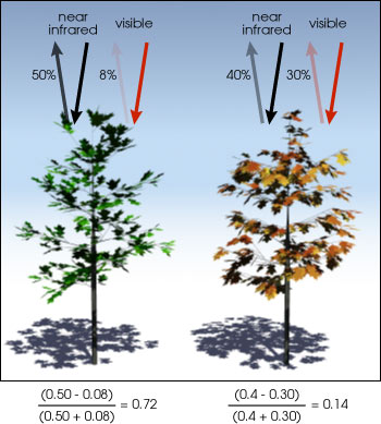
A vegetation index is a single value that quantifies vegetation health or structure. The math associated with calculating a vegetation index is derived from the physics of light reflection and absorption across bands. For instance, it is known that healthy vegetation reflects light strongly in the near infrared band and less strongly in the visible portion of the spectrum. Thus, if you create a ratio between light reflected in the near infrared and light reflected in the visible spectrum, it will represent areas that potentially have healthy vegetation.

Normalized Difference Vegetation Index (NDVI)

The Normalized Difference Vegetation Index (NDVI) is a quantitative index of greenness ranging from 0-1, where 0 represents minimal or no greenness and 1 represents maximum greenness.

NDVI is often used for a quantitate proxy measure of vegetation health, cover and phenology (life cycle stage) over large areas.

NDVI image from NASA that shows reflectance. — NDVI is calculated from the visible and near-infrared light reflected by vegetation. Healthy vegetation (left) absorbs most of the visible light that hits it, and reflects a large portion of near-infrared light. Unhealthy or sparse vegetation (right) reflects more visible light and less near-infrared light. Source: NASA Earth Observatory

More on NDVI from NASA

Calculate NDVI in R

Sometimes you can download already calculated NDVI data products. In this case, you need to calculate NDVI using the NAIP imagery / reflectance data that you have.

# load spatial packages
library(raster)
library(rgdal)
library(rgeos)
library(RColorBrewer)

# turn off factors
options(stringsAsFactors = FALSE)

# import the naip pre-fire data
naip_multispectral_st <- stack("data/week-07/naip/m_3910505_nw_13_1_20130926/crop/m_3910505_nw_13_1_20130926_crop.tif")

# convert data into rasterbrick for faster processing
naip_multispectral_br <- brick(naip_multispectral_st)

How to Derive the NDVI Vegetation Index

The normalized difference vegetation index (NDVI) uses a ratio between near infrared and red light within the electromagnetic spectrum. To calculate NDVI, you use the following formula where NIR is near infrared light and red represents red light. For your raster data, you will take the reflectance value in the red and near infrared bands to calculate the index.

(NIR - Red) / (NIR + Red)

# calculate ndvi with naip
naip_multispectral_br[[4]]
## class      : RasterLayer 
## dimensions : 2312, 4377, 10119624  (nrow, ncol, ncell)
## resolution : 1, 1  (x, y)
## extent     : 457163, 461540, 4424640, 4426952  (xmin, xmax, ymin, ymax)
## crs        : +proj=utm +zone=13 +ellps=GRS80 +towgs84=0,0,0,0,0,0,0 +units=m +no_defs 
## source     : memory
## names      : m_3910505_nw_13_1_20130926_crop.4 
## values     : 0, 255  (min, max)

# calculate NDVI using the red (band 1) and nir (band 4) bands
naip_ndvi <- (naip_multispectral_br[[4]] - naip_multispectral_br[[1]]) / (naip_multispectral_br[[4]] + naip_multispectral_br[[1]])

# plot the data
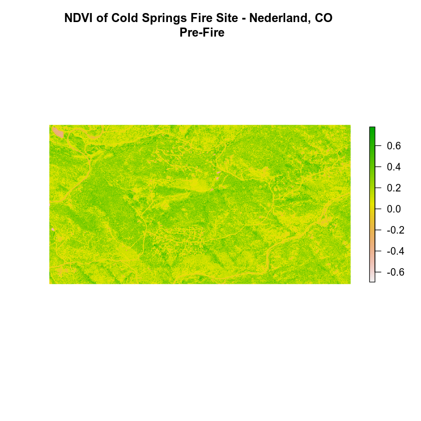
plot(naip_ndvi,
     main = "NDVI of Cold Springs Fire Site - Nederland, CO \n Pre-Fire",
     axes = FALSE, box = FALSE)

NAIP derived NDVI plot.

View Distribution of NDVI Values

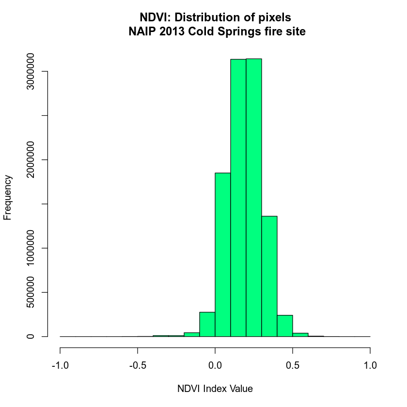
# view distribution of NDVI values
hist(naip_ndvi,
  main = "NDVI: Distribution of pixels\n NAIP 2013 Cold Springs fire site",
  col = "springgreen",
  xlab = "NDVI Index Value")

Histogram of NAIP derived NDVI.

Export Raster

When you are done, you may want to export your rasters so you can use them in QGIS or ArcGIS or share them with your colleagues. To do this you use the writeRaster() function.

# Check if the directory exists using the function you created last week
check_create_dir("data/week-07/outputs/")

# Export your raster
writeRaster(x = naip_ndvi,
              filename="data/week-07/outputs/naip_ndvi_2013_prefire.tif",
              format = "GTiff", # save as a tif
              datatype='INT2S', # save as a INTEGER rather than a float
              overwrite = TRUE)  # OPTIONAL - be careful. This will OVERWRITE previous files.

Faster Raster Calculations with the Overlay Function

You can perform raster calculations using raster math as you did above. However, it’s much more efficient and faster to use the overlay() function in R. To use the overlay function you provide R with:

The bands or raster layers that you want it to use for some calculation.
A function that you create or provide that you want to run on those bands.

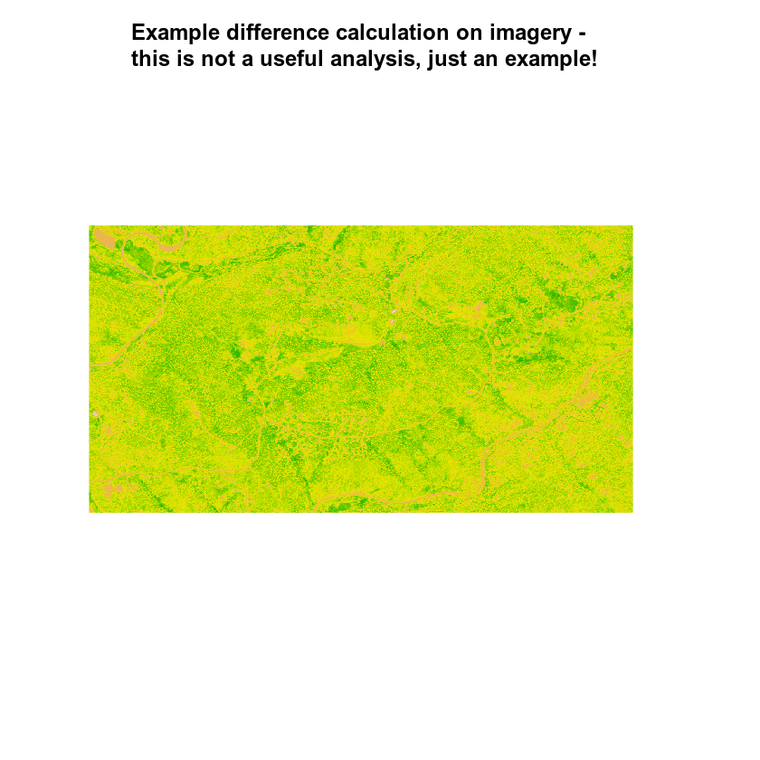
Let’s look at an example below where you simply subtract two layers using overlay(). You could use this same function to subtract rasters (like you did to create the canopy height models and the different rasters in week 3).

# create a function that subtracts two rasters

diff_rasters <- function(b1, b2){
  # this function calculates the difference between two rasters of the same CRS and extent
  # input: 2 raster layers of the same extent, crs that can be subtracted
  # output: a single different raster of the same extent, crs of the input rasters
  diff <- b2 - b1
  return(diff)
}

Now, use the overlay function to subtract two rasters.

band_diff <- overlay(naip_multispectral_br[[1]], naip_multispectral_br[[4]],
        fun = diff_rasters)

plot(band_diff,
     main = "Example difference calculation on imagery - \n this is not a useful analysis, just an example!",
     axes = FALSE, box = FALSE, legend = FALSE)

Example plot of band difference.

# calculate ndvi using the overlay function
# you will have to create the function on your own!
naip_ndvi_ov <- overlay(naip_multispectral_br[[1]],
        naip_multispectral_br[[4]],
        fun = normalized_diff)

plot(naip_ndvi_ov,
     main = "NAIP NDVI calculated using the overlay function")

NAIP derived NDVI plot using overlay function.

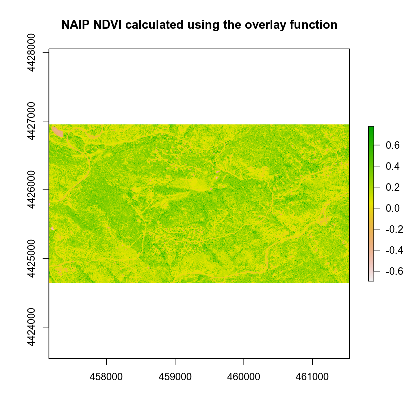
Don’t believe overlay is faster? Let’s test it using a benchmark.

library(microbenchmark)
# is the raster in memory?
inMemory(naip_multispectral_st)
## [1] FALSE

# How long does it take to calculate ndvi without overlay.
microbenchmark((naip_multispectral_br[[4]] - naip_multispectral_br[[1]]) / (naip_multispectral_br[[4]] + naip_multispectral_br[[1]]), times = 10)
## Unit: milliseconds
##                                                                                                                      expr
##  (naip_multispectral_br[[4]] - naip_multispectral_br[[1]])/(naip_multispectral_br[[4]] +      naip_multispectral_br[[1]])
##       min       lq     mean   median       uq    max neval
##  475.3372 511.7044 531.0472 537.4337 553.2409 566.75    10

# is a raster brick faster?
microbenchmark(overlay(naip_multispectral_br[[1]],
        naip_multispectral_br[[4]],
        fun = normalized_diff), times = 10)
## Unit: milliseconds
##                                                                                         expr
##  overlay(naip_multispectral_br[[1]], naip_multispectral_br[[4]],      fun = normalized_diff)
##       min       lq     mean   median       uq      max neval
##  403.1773 418.5548 498.6839 464.9501 476.3928 733.5285    10

Notice that the results above suggest that the overlay function is in fact just a bit faster than the regular raster math approach. This may seem minor now. However, you are only working with 55mb files. This will save processing time in the long run as you work with larger raster files.

In the next lesson, you will find a few sets of tests on raster processing speed.

Additional Resources

Faster Raster Calculations Additive Color Models

Share on

Twitter Facebook Google+ LinkedIn

Earth Data Analytics Online Certificate

Earth analytics

earth-analytics Home