Lesson 3. Plot Grid of Spatial Plots in R.
Learning Objectives
After completing this tutorial, you will be able to:
- Plot several plots using baseplot functions in a “grid” as one graphic in
R.
What You Need
You will need a computer with internet access to complete this lesson and the data for week 8 of the course.
# load libraries
library(raster)
library(rgeos)
library(rgdal)
# import landsat data
all_landsat_bands <- list.files("data/week-08/landsat/LC80340322016189-SC20170128091153/crop",
           pattern = glob2rx("*band*.tif$"),
           full.names = TRUE) # use the dollar sign at the end to get all files that END WITH

all_landsat_bands_st <- stack(all_landsat_bands)
Creating a Grid of Plots
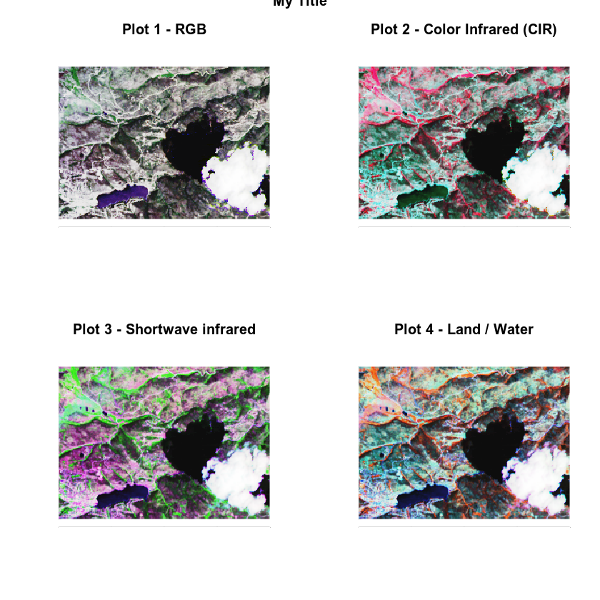
You can plot several plots together in the same window using baseplot. To do this, you use the parameter value mfrow=c(x,y) where x is the number of rows that you wish to have in your plot and y is the number of columns. When you plot, R will place each plot, in order by row within the grid that you define using mfrow.
Below, you have created a 2 by 2 grid of plots using mfrow=c(2,2) within the par() function. In this example you have 2 rows and 2 columns.
# adjust the parameters so the axes colors are white. Also turn off tick marks.
par(mfrow = c(2,2), col.axis = "white", col.lab = "white", tck = 0)
# plot 1
plotRGB(all_landsat_bands_st,
        r = 4,g = 3,b = 2,
        stretch = "hist",
        main = "Plot 1 - RGB",
        axes = TRUE)
box(col = "white") # turn all of the lines to white

# plot 2
plotRGB(all_landsat_bands_st,
        r = 5,g = 4,b = 3,
        stretch = "hist",
        main = "Plot 2 - Color Infrared (CIR)",
        axes = TRUE)
box(col = "white") # turn all of the lines to white

# plot 3
plotRGB(all_landsat_bands_st,
        r = 7,g = 5,b = 4,
        stretch = "hist",
        main = "Plot 3 - Shortwave infrared",
        axes = TRUE)
box(col = "white") # turn all of the lines to white

# plot 4
plotRGB(all_landsat_bands_st,
        r = 5,g = 6,b = 4,
        stretch = "hist",
        main = "Plot 4 - Land / Water",
        axes = TRUE)
# set bounding box to white as well
box(col = "white") # turn all of the lines to white

# add overall title to your layout
title("My Title", outer = TRUE)

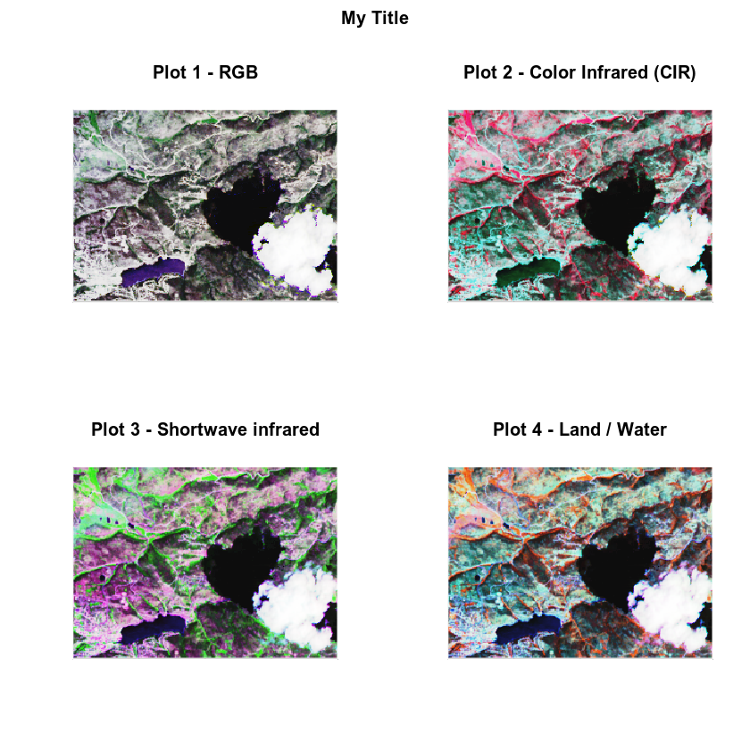
Above, you added an overall title to your grid of plots using the title() function. However the title is chopped of because there is not enough of a margin at the top for it. You can adjust for this too using the oma= parameter argument. oma sets the outside (o) margin (ma).
oma= argument in your par() function. Let’s try it.
# adjust the parameters so the axes colors are white. Also turn off tick marks.
par(mfrow = c(2,2), oma = c(0,0,2,0), col.axis = "white", col.lab = "white", tck = 0)
# plot 1
plotRGB(all_landsat_bands_st,
        r = 4,g = 3,b = 2,
        stretch = "hist",
        main = "Plot 1 - RGB",
        axes = TRUE)
box(col = "white") # turn all of the lines to white

# plot 2
plotRGB(all_landsat_bands_st,
        r = 5,g = 4,b = 3,
        stretch = "hist",
        main = "Plot 2 - Color Infrared (CIR)",
        axes = TRUE)
box(col = "white") # turn all of the lines to white

# plot 3
plotRGB(all_landsat_bands_st,
        r = 7,g = 5,b = 4,
        stretch = "hist",
        main = "Plot 3 - Shortwave infrared",
        axes = TRUE)
box(col = "white") # turn all of the lines to white

# plot 4
plotRGB(all_landsat_bands_st,
        r = 5,g = 6,b = 4,
        stretch = "hist",
        main = "Plot 4 - Land / Water",
        axes = TRUE)
# set bounding box to white as well
box(col = "white") # turn all of the lines to white

# add overall title to your layout
title("My Title", outer = TRUE)

When you are done with plotting in a grid space, be sure to reset your plot space using dev.off().
dev.off()
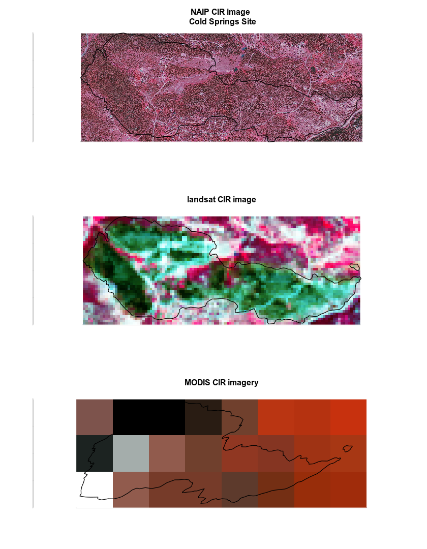
Your homework this week should look something like this:

Share on
Twitter Facebook Google+ LinkedIn
Leave a Comment