Lesson 4. Adjust plot extent in R.
Learning Objectives
After completing this tutorial, you will be able to:
- Adjust the spatial extent of a plot using the
ext=argument in R.
What you need
You will need a computer with internet access to complete this lesson and the data for week 8 of the course.
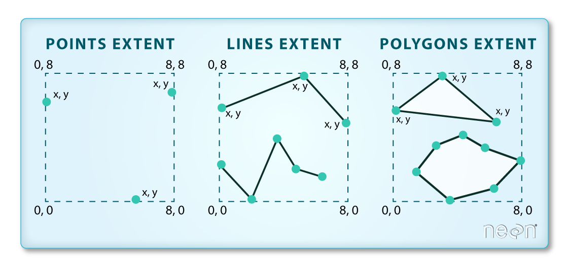
Review: What is an extent?
all_landsat_bands <- list.files("data/week-08/landsat/LC80340322016189-SC20170128091153/crop",
           pattern = glob2rx("*band*.tif$"),
           full.names = TRUE) # use the dollar sign at the end to get all files that END WITH

all_landsat_bands_st <- stack(all_landsat_bands)

# turn the axis color to white and turn off ticks
par(col.axis = "white", col.lab = "white", tck = 0)
# plot the data - be sure to turn AXES to T (you just color them white)
plotRGB(all_landsat_bands_st,
        r = 4, g = 3, b = 2,
        stretch = "hist",
        main = "Pre-fire RGB image with cloud\n Cold Springs Fire",
        axes = TRUE)
# turn the box to white so there is no border on your plot
box(col = "white")

Adjust plot extent
You can adjust the extent of a plot using ext argument. You can give the argument the spatial extent of the fire boundary layer that you want to plot.
If your object is called fire_boundary_utm, then you’d code: ext=extent(fire_boundary_utm)
# import fire overlay boundary
fire_boundary <- readOGR("data/week-08/vector_layers/fire-boundary-geomac/",
                         "co_cold_springs_20160711_2200_dd83")
## OGR data source with driver: ESRI Shapefile
## Source: "/root/earth-analytics/data/week-08/vector_layers/fire-boundary-geomac", layer: "co_cold_springs_20160711_2200_dd83"
## with 1 features
## It has 21 fields
# reproject the data
fire_boundary_utm <- spTransform(fire_boundary, CRS = crs(all_landsat_bands_st))

# turn the axis color to white and turn off ticks
par(col.axis = "white", col.lab = "white", tck = 0)
# plot the data - be sure to turn AXES to T (you just color them white)
plotRGB(all_landsat_bands_st,
        r = 4, g = 3, b = 2,
        stretch = "hist",
        main = "Pre-fire RGB image with cloud\n Cold Springs Fire\n Fire boundary extent",
        axes = TRUE,
        ext = extent(fire_boundary_utm))
# turn the box to white so there is no border on your plot
box(col = "white")
plot(fire_boundary_utm, add = TRUE)

Share on
Twitter Facebook Google+ LinkedIn
Leave a Comment