Lesson 3. How to Replace Raster Cell Values with Values from A Different Raster Data Set in R
Learning Objectives
After completing this tutorial, you will be able to:
- Use the cover function in R to replace missing or bad data values in a raster with values from another raster
What You Need
You will need a computer with internet access to complete this lesson and the data for week 8 of the course.
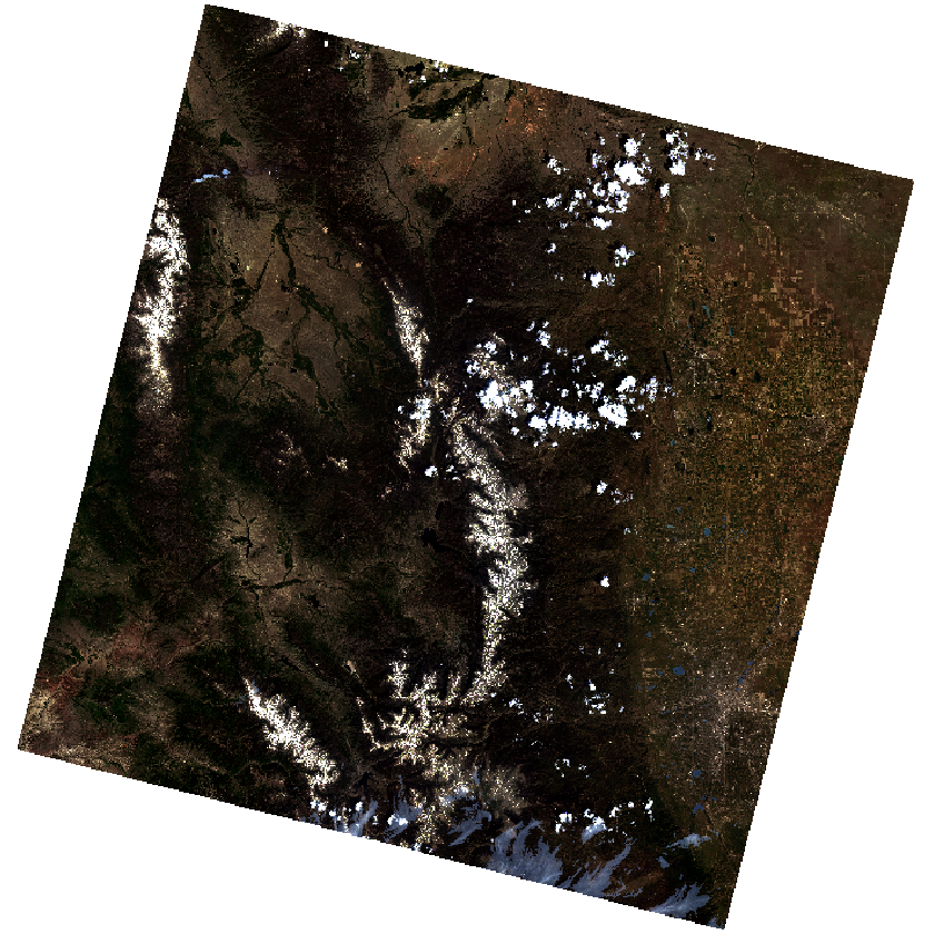
First, import and stack the “cleaner” better Landsat data. Convert it to a rasterbrick.
# import data with less cloud cover
all_landsat_bands_pre_nocloud <- list.files("data/week-08/landsat/LC80340322016173-SC20170227185411",
                                pattern = glob2rx("*band*.tif$"),
                                full.names = TRUE) # use the dollar sign at the end to get all files that END WITH

all_landsat_bands_pre_nocloud_st <- stack(all_landsat_bands_pre_nocloud)
all_landsat_bands_pre_nocloud_br <- stack(all_landsat_bands_pre_nocloud_st)
plotRGB(all_landsat_bands_pre_nocloud_br,
        r = 4, g = 3, b = 2,
        stretch = 'lin')

# import the data with the clouds
# create a list of all landsat files that have the extension .tif and contain the word band.
all_landsat_bands_cloudy <- list.files("data/week-08/landsat/LC80340322016189-SC20170128091153/crop",
           pattern = glob2rx("*band*.tif$"),
           full.names = TRUE)

# create spatial raster stack from the list of file names
all_landsat_bands_cloudy_st <- stack(all_landsat_bands_cloudy)
all_landsat_bands_cloudy_br <- brick(all_landsat_bands_cloudy_st)
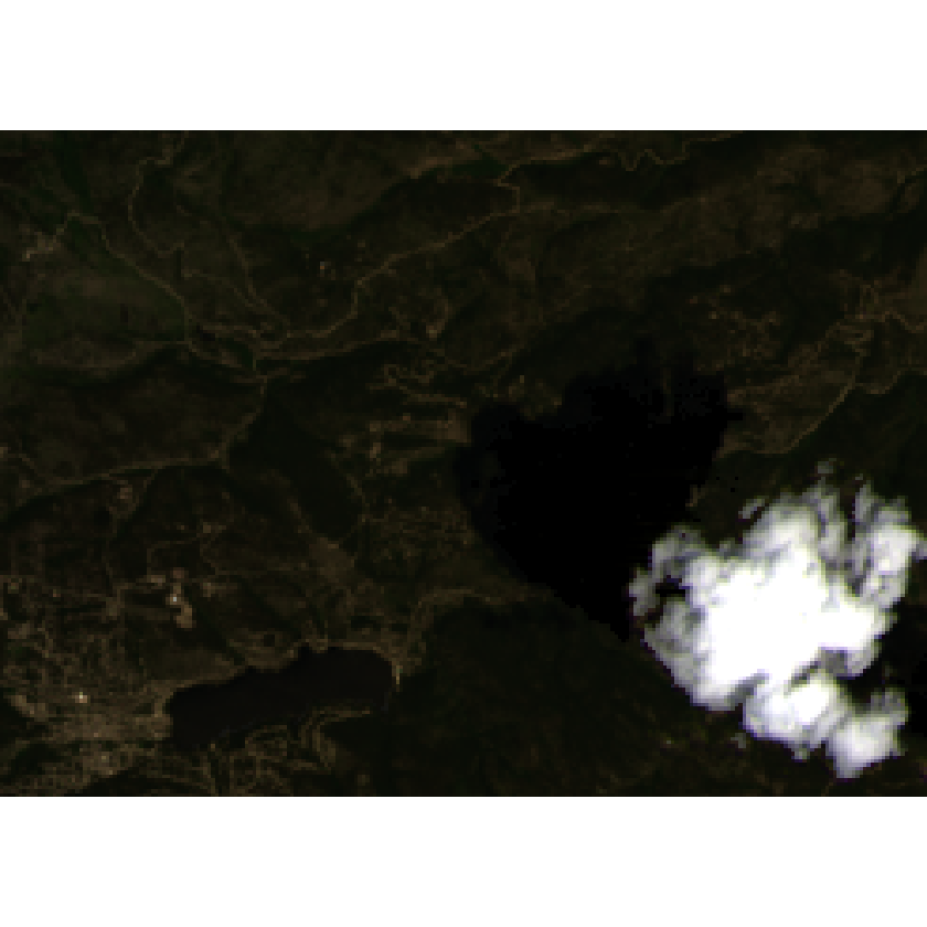
plotRGB(all_landsat_bands_cloudy_br,
        r = 4, g = 3, b = 2,
        stretch = "lin")

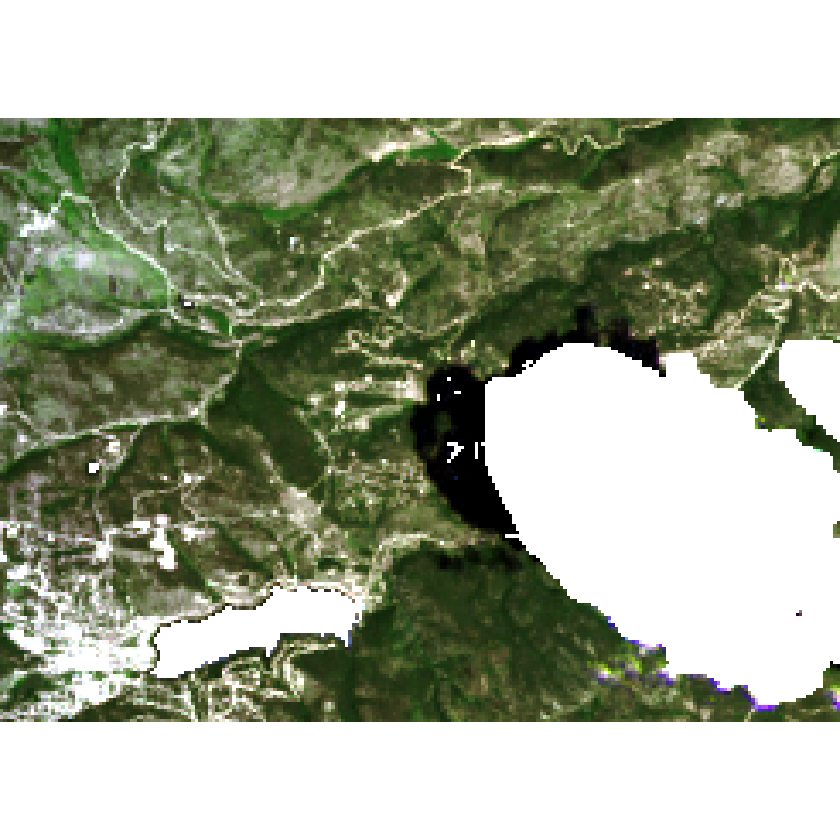
Apply the cloud mask to the cloudy data.
# open cloud mask layer
cloud_mask_189 <- raster("data/week-08/landsat/LC80340322016189-SC20170128091153/crop/LC80340322016189LGN00_cfmask_crop.tif")

cloud_mask_189[cloud_mask_189 > 0] <- NA

all_landsat_bands_mask <- mask(all_landsat_bands_cloudy_br,
                               mask = cloud_mask_189)
plotRGB(all_landsat_bands_mask,
        r = 4, g = 3, b = 2,
        stretch = "lin")

Check to see if the rasters are in the same extent and CRS.
compareRaster(all_landsat_bands_pre_nocloud_br, all_landsat_bands_mask)
## Error in compareRaster(all_landsat_bands_pre_nocloud_br, all_landsat_bands_mask): different extent
The extents are different, let’s crop one to the other.
all_landsat_bands_pre_nocloud_br <- crop(all_landsat_bands_pre_nocloud_br, extent(all_landsat_bands_cloudy_br))

# are they in the same extent now?
compareRaster(all_landsat_bands_pre_nocloud_br, all_landsat_bands_mask)
## [1] TRUE
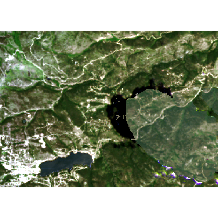
Use the cover() function to replace each pixel that has an assigned NA value with the pixel reflectance value in the same band in the other raster.
# crop the data using the extend of the other raster
cleaned_raster <- cover(all_landsat_bands_mask, all_landsat_bands_pre_nocloud_br)
plotRGB(cleaned_raster, r = 4, g = 3, b = 2, stretch = 'lin')

Things are looking a bit better but still this image has issues:
- There are edge effects associated with the mask that you can see.
- Shadows weren’t handled well with that mask.
You might have more processing to do to truly get this image cleaned up.
In this case, it could be better to use the other image in your analysis rather than trying to clean up the cloud image.
Share on
Twitter Facebook Google+ LinkedIn
Leave a Comment