This lesson introduces the data.frame which is very similar to working with a spreadsheet in R.

In the homework from week 1, you used the code below to create a report with knitr in RStudio.

# load the ggplot2 library for plotting
library(ggplot2)

# turn off factors
options(stringsAsFactors = FALSE)

# download data from figshare
download.file("https://ndownloader.figshare.com/files/9282364",
              "data/boulder-precip.csv",
              method = "libcurl")

Let’s break the code above down. First, you use the download.file function to download a datafile. In this case, the data are housed on Figshare - a popular data repository that is free to use if your data are cumulatively smaller than 20gb.

Notice that download.file() function has two ARGUMENTS:

1. url: this is the path to the data file that you wish to download.
2. destfile: this is the location on your computer (in this case: /data) and name of the file when saved (in this case: boulder-precip.csv). So you downloaded a file from a url on figshare to your data directory. You named that file boulder-precip.csv.

Next, you read in the data using the function: read.csv().

# import data
boulder_precip <- read.csv(file = "data/boulder-precip.csv")

# view first few rows of the data
head(boulder_precip)
##     X       DATE PRECIP
## 1 756 2013-08-21    0.1
## 2 757 2013-08-26    0.1
## 3 758 2013-08-27    0.1
## 4 759 2013-09-01    0.0
## 5 760 2013-09-09    0.1
## 6 761 2013-09-10    1.0

# view the format of the boulder_precip object in R
str(boulder_precip)
## 'data.frame':	18 obs. of  3 variables:
##  $ X     : int  756 757 758 759 760 761 762 763 764 765 ...
##  $ DATE  : chr  "2013-08-21" "2013-08-26" "2013-08-27" "2013-09-01" ...
##  $ PRECIP: num  0.1 0.1 0.1 0 0.1 1 2.3 9.8 1.9 1.4 ...

Introduction to the Data Frame

When you read data into R using read.csv() it imports it into a data frame format. Data frames are the de facto data structure for most tabular data, and what you use for statistics and plotting.

A data.frame is a collection of vectors of identical lengths. Each vector represents a column, and each vector can be of a different data type (e.g. characters, integers, factors). The str() function is useful to inspect the data types of the columns.

A data.frame can be created by hand but most commonly they are generated when you import a text file or spreadsheet into R using the functions read.csv() or read.table().

Extracting / Specifying “Columns” by Name

You can extract just one single column from your data.frame using the $ symbol followed by the name of the column (or the column header):

# when you download the data you create a data.frame
# view each column of the data frame using its name (or header)
boulder_precip$DATE
##  [1] "2013-08-21" "2013-08-26" "2013-08-27" "2013-09-01" "2013-09-09"
##  [6] "2013-09-10" "2013-09-11" "2013-09-12" "2013-09-13" "2013-09-15"
## [11] "2013-09-16" "2013-09-22" "2013-09-23" "2013-09-27" "2013-09-28"
## [16] "2013-10-01" "2013-10-04" "2013-10-11"

# view the precip column
boulder_precip$PRECIP
##  [1] 0.1 0.1 0.1 0.0 0.1 1.0 2.3 9.8 1.9 1.4 0.4 0.1 0.3 0.3 0.1 0.0 0.9
## [18] 0.1

View Structure of a Data Frame

You can explore the format of your data frame in a similar way to how you explored vectors in the third lesson of this module. Let’s take a look.

# when you download the data you create a data.frame
# view each column of the data frame using its name (or header)
# how many rows does the data frame have
nrow(boulder_precip)
## [1] 18

# view the precip column
boulder_precip$PRECIP
##  [1] 0.1 0.1 0.1 0.0 0.1 1.0 2.3 9.8 1.9 1.4 0.4 0.1 0.3 0.3 0.1 0.0 0.9
## [18] 0.1

Plotting Your Data

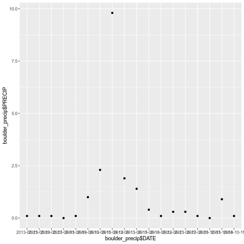
YOu can quickly plot your data too. Note that you are using the ggplot2 function qplot() rather than the R base plot functionality. You are doing this because ggplot2 is generally more powerful and efficient to use for plotting.

# q plot stands for quick plot. Let's use it to plot your data
qplot(x = boulder_precip$DATE,
      y = boulder_precip$PRECIP)