This lesson briefly discusses the key differences between projected vs. geographic coordinate reference systems.

Geographic vs Projected CRS

In the previous tutorial, you explored the basic concept of a coordinate reference system. During the lesson you looked at two different types of Coordinate Reference Systems:

1. Geographic coordinate systems: coordinate systems that span the entire globe (e.g. latitude / longitude).
2. Projected coordinate systems: coordinate systems that are localized to minimize visual distortion in a particular region (e.g. Robinson, UTM, State Plane)

In this tutorial, you will learn the differences between these CRS’s in more detail.

As you learned in the previous lesson, each CRS is optimized to best represent the:

• shape and/or
• scale / distance and/or
• area

of features in a dataset. There is not a single CRS that does a great job at optimizing all three elements: shape, distance AND area. Some CRSs are optimized for shape, some are optimized for distance and some are optimized for area. Some CRS’s are also optimized for particular regions, for instance the United States, or Europe.

Intro to Geographic Coordinate Reference Systems

Geographic coordinate systems (which are often but not always in decimal degree units) are often optimal when you need to locate places on the Earth. Or when you need to create global maps. However, latitude and longitude locations are not located using uniform measurement units. Thus, geographic CRS’s are not ideal for measuring distance. This is why other projected CRS have been developed.

The Structure of a Geographic CRS

A geographic CRS uses a grid that wraps around the entire globe. This means that each point on the globe is defined using the SAME coordinate system and the same units as defined within that particular geographic CRS. Geographic coordinate reference systems are best for global analysis however it is important to remember that distance is distorted using a geographic lat / long CRS.

The geographic WGS84 lat/long CRS has an origin - (0,0) - located at the intersection of the Equator (0° latitude) and Prime Meridian (0° longitude) on the globe.

Let’s remind ourselves what data projects in a geographic CRS look like.

library(ggplot2)
library(rgdal)
library(raster)

Data Note: The distance between the 2 degrees of longitude at the equator (0°) is ~ 69 miles. The distance between 2 degrees of longitude at 40°N (or S) is only 53 miles. This difference in actual distance relative to “distance” between the actual parallels and meridians demonstrates how distance calculations will be less accurate when using geographic CRS’s

Projected Coordinate Reference Systems

As you learned above, geographic coordinate systems are ideal for creating global maps. However, they are prone to error when quantifying distance. In contrast, various spatial projections have evolved that can be used to more accurately capture distance, shape and/or area.

What is a Spatial Projection

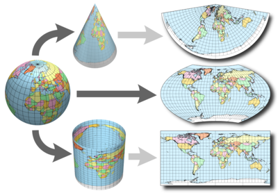
Spatial projection refers to the mathematical calculations performed to flatten the 3D data onto a 2D plane (your computer screen or a paper map). Projecting data from a round surface onto a flat surface results in visual modifications to the data when plotted on a map. Some areas are stretched and some some are compressed. You can see this distortion when you look at a map of the entire globe.

The mathematical calculations used in spatial projections are designed to optimize the relative size and shape of a particular region on the globe.

About UTM

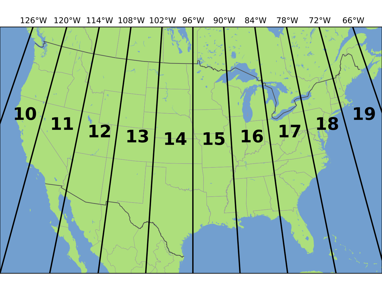
The Universal Transverse Mercator (UTM) system is a commonly used projected coordinate reference system. UTM subdivides the globe into zones, numbered 0-60 (equivalent to longitude) and regions (north and south).

Data Note: UTM zones are also defined using bands, lettered C-X (equivalent to latitude) however, the band designation is often dropped as it isn’t essential to specifying the location.

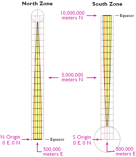
While UTM zones span the entire globe, UTM uses a regional projection and associated coordinate system. The coordinate system grid for each zone is projected individually using the Mercator projection.

The origin (0,0) for each UTM zone and associated region is located at the intersection of the equator and a location, 500,000 meters east of the central meridian of each zone. The origin location is placed outside of the boundary of the UTM zone, to avoid negative Easting numbers.

Understand UTM Coordinates

Let’s compare coordinates for one location, but saved in two different CRS’s to better understand what this looks like. The coordinates for Boulder, Colorado in UTM are:

UTM Zone 13N easting: 476,911.31m, northing: 4,429,455.35

Remember that N denotes that it is in the Northern hemisphere on the Earth.

Let’s plot this coordinate on a map.

# create a data.frame with the x,y location
boulder_df <- data.frame(lon = c(476911.31),
                lat = c(4429455.35))

# plot boulder
ggplot() +
                geom_point(data = boulder_df,
                aes(x = lon, y = lat, group = NULL), colour = "springgreen",
                      size = 5)

# convert to spatial points
coordinates(boulder_df) <- 1:2

class(boulder_df)
## [1] "SpatialPoints"
## attr(,"package")
## [1] "sp"
crs(boulder_df)
## CRS arguments: NA

# assign crs - you know it is utm zone 13N
crs(boulder_df) <- CRS("+init=epsg:2957")

Note what the projection string for your data in UTM looks like: +init=epsg:2957 +proj=utm +zone=13 +ellps=GRS80 +towgs84=0,0,0,0,0,0,0 +units=m +no_defs

If you spatially project your data into a geographic coordinate reference system, notice how your new coordinates are different - yet they still represent the same location.

boulder_df_geog <- spTransform(boulder_df, crs(worldBound))
coordinates(boulder_df_geog)
##            lon      lat
## [1,] -105.2705 40.01498

Now you can plot your data on top of your world map which is also in a geographic CRS.

boulder_df_geog <- as.data.frame(coordinates(boulder_df_geog))
# plot map
worldMap <- ggplot(worldBound_df, aes(long,lat, group = group)) +
  geom_polygon() +
  xlab("Longitude (Degrees)") + ylab("Latitude (Degrees)") +
  coord_equal() +
  ggtitle("Global Map - Geographic Coordinate System - WGS84 Datum\n Units: Degrees - Latitude / Longitude")

# map boulder
worldMap +
        geom_point(data = boulder_df_geog,
        aes(x = lon, y = lat, group = NULL), colour = "springgreen", size = 5)

Important

While sometimes UTM zones in the north vs south are specified using N and S respectively (e.g. UTM Zone 18N) other times you may see a letter as follows: Zone 18T, 730782m Easting, 4712631m Northing vs UTM Zone 18N, 730782m, 4712631m.

Data Tip: The UTM system doesn’t apply to polar regions (>80°N or S). Universal Polar Stereographic (UPS) coordinate system is used in these area. This is where zones A, B and Y, Z are used if you were wondering why they weren’t in the UTM lettering system.

Datum

The datum describes the vertical and horizontal reference point of the coordinate system. The vertical datum describes the relationship between a specific ellipsoid (the top of the earth’s surface) and the center of the earth. The datum also describes the origin (0,0) of a coordinate system.

Frequently encountered datums:

• WGS84 – World Geodetic System (created in) 1984. The origin is the center of the Earth.
• NAD27 & NAD83 – North American Datum 1927 and 1983, respectively. The origin for NAD 27 is Meades Ranch in Kansas.
• ED50 – European Datum 1950

NOTE: All coordinate reference systems have a vertical and horizontal datum which defines a “0, 0” reference point. There are two models used to define the datum: ellipsoid (or spheroid): a mathematically representation of the shape of the earth. Visit Wikipedia’s article on the earth ellipsoid for more information and geoid: a model of the Earth’s gravitatinal field which approximates the mean sea level across the entire Earth. It is from this that elevation is measured. Visit Wikipedia’s geoid article for more information. You will not learn these concepts in this tutorial.

Coordinate Reference System Formats

There are numerous formats that are used to document a CRS. In the next tutorial you will learn three of the commonly encountered formats including: Proj4, WKT (Well Known Text) and EPSG.