Lesson 6. Work with MODIS Remote Sensing Data in R.
Learning Objectives
After completing this tutorial, you will be able to:
- Open MODIS imagery in
R. - Create NBR index using MODIS imagery in
R. - Calculate total burned area in
R.
What You Need
You will need a computer with internet access to complete this lesson and the data for week 8 of the course.
First, let’s import MODIS data. Below notice that you have used a slightly different version of the list.files() pattern = argument.
You have used glob2rx("*sur_refl*.tif$") to select all layers that both
- Contain the word
sur_reflin them and - Contain the extension
.tif
Let’s import your MODIS image stack.
# open modis bands (layers with sur_refl in the name)
all_modis_bands_july7 <- list.files("data/week-08/modis/reflectance/07_july_2016/crop",
           pattern = glob2rx("*sur_refl*.tif$"),
           full.names = TRUE)
# create spatial raster stack
all_modis_bands_pre_st <- stack(all_modis_bands_july7)
all_modis_bands_pre_br <- brick(all_modis_bands_pre_st)

# view range of values in stack
all_modis_bands_pre_br[[2]]
## class      : RasterLayer
## dimensions : 2400, 2400, 5760000  (nrow, ncol, ncell)
## resolution : 463.3127, 463.3127  (x, y)
## extent     : -10007555, -8895604, 3335852, 4447802  (xmin, xmax, ymin, ymax)
## crs        : +proj=sinu +lon_0=0 +x_0=0 +y_0=0 +a=6371007.181 +b=6371007.181 +units=m +no_defs
## source     : memory
## names      : MOD09GA.A2016189.h09v05.006.2016191073856_sur_refl_b02_1
## values     : -1000000, 100390000  (min, max)

# view band names
names(all_modis_bands_pre_br)
## [1] "MOD09GA.A2016189.h09v05.006.2016191073856_sur_refl_b01_1"
## [2] "MOD09GA.A2016189.h09v05.006.2016191073856_sur_refl_b02_1"
## [3] "MOD09GA.A2016189.h09v05.006.2016191073856_sur_refl_b03_1"
## [4] "MOD09GA.A2016189.h09v05.006.2016191073856_sur_refl_b04_1"
## [5] "MOD09GA.A2016189.h09v05.006.2016191073856_sur_refl_b05_1"
## [6] "MOD09GA.A2016189.h09v05.006.2016191073856_sur_refl_b06_1"
## [7] "MOD09GA.A2016189.h09v05.006.2016191073856_sur_refl_b07_1"

# clean up the band names for neater plotting
names(all_modis_bands_pre_br) <- gsub("MOD09GA.A2016189.h09v05.006.2016191073856_sur_refl_b", "Band",
     names(all_modis_bands_pre_br))

# view cleaned up band names
names(all_modis_bands_pre_br)
## [1] "Band01_1" "Band02_1" "Band03_1" "Band04_1" "Band05_1" "Band06_1"
## [7] "Band07_1"
Reflectance Values Range 0-1
As you’ve learned in class, the normal range of reflectance values is 0-1 where 1 is the BRIGHTEST values and 0 is the darkest value. Have a close look at the min and max values in the second raster layer of your stack, above. What do you notice?
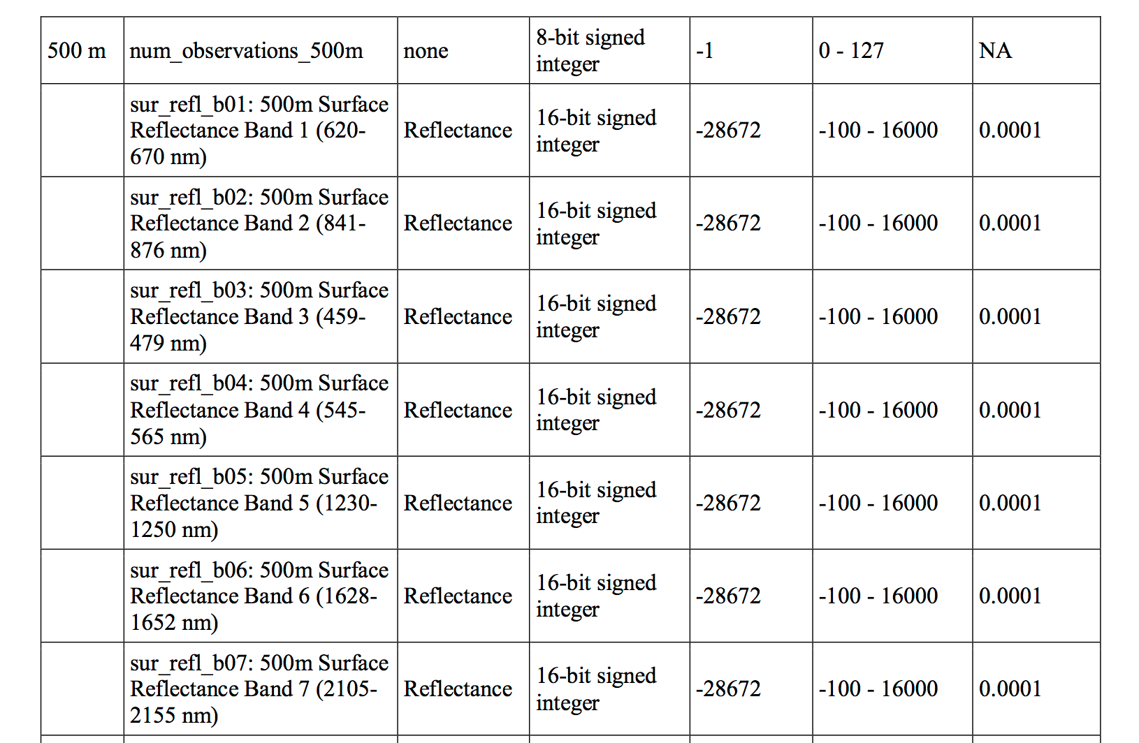
The min and max values are widely outside of the expected range of 0-1 - min: -32768, max: 32767 What could be causing this? You need to better understand your data before you can work with it more. Have a look at the table in the MODIS users guide. The data that you are working with is the MOD09GA product. Look closely at the table on page 14 of the guide. Part of the table can be seen below.
Click here to check out the MODIS user guide - check out page 14 for the MOD09GA table.
The column headings for the table below:
| Group | Science Data Sets (HDF Layers (21)) | Units | Data Type | Fill Value | Valid Range | Scale Factor |
|---|---|---|---|---|---|---|
| surf_Refl_b01: 500m Surface Reflectance Band 1 (620-670 nm) | Reflectance | 16-bit signed integer | -28672 | -100 - 16000 | 0.0001 | |
| surf_Refl_b02: 500m Surface Reflectance Band 2 (841-876 nm) | Reflectance | 16-bit signed integer | -28672 | -100 - 16000 | 0.0001 | |
| surf_Refl_b03: 500m Surface Reflectance Band 3 (459-479 nm) | Reflectance | 16-bit signed integer | -28672 | -100 - 16000 | 0.0001 | |
| surf_Refl_b04: 500m Surface Reflectance Band 4 (545-565 nm) | Reflectance | 16-bit signed integer | -28672 | -100 - 16000 | 0.0001 | |
| surf_Refl_b05: 500m Surface Reflectance Band 5 (1230-1250 nm) | Reflectance | 16-bit signed integer | -28672 | -100 - 16000 | 0.0001 | |
| surf_Refl_b06: 500m Surface Reflectance Band 6 (1628-1652 nm) | Reflectance | 16-bit signed integer | -28672 | -100 - 16000 | 0.0001 | |
| surf_Refl_b07: 500m Surface Reflectance Band 7 (2105-2155 nm) | Reflectance | 16-bit signed integer | -28672 | -100 - 16000 | 0.0001 |
Looking at the table, answer the following questions
- What is valid range of values for your data?
- What is the scale factor associated with your data?
Explore Your Data
Looking at histograms of your data, you can see that the range of values is not what you’d expect. You’d expect values between -100 to 10000 yet instead you have much larger numbers.
# turn off scientific notation
options("scipen" = 100, "digits" = 4)
# bottom, left, top and right
#par(mfrow=c(4, 2))
hist(all_modis_bands_pre_br,
  col = "springgreen",
  xlab = "Reflectance Value")
mtext("Distribution of MODIS reflectance values for each band\n Data not scaled",
      outer = TRUE, cex = 1.5)

Scale Factor
Looking at the metadata, you can see that your data have a scale factor. Let’s deal with that before doing anything else. The scale factor is .0001. This means you should multiple each layer by that value to get the actual reflectance values of the data.
You can apply this math to all of the layers in your stack using a simple calculation shown below:
# deal with nodata value --  -28672
all_modis_bands_pre_br <- all_modis_bands_pre_br * .0001
# view histogram of each layer in your stack
# par(mfrow=c(4, 2))
hist(all_modis_bands_pre_br,
   xlab = "Reflectance Value",
   col = "springgreen")
mtext("Distribution of MODIS reflectance values for each band\n Scale factor applied", outer = TRUE, cex = 1.5)

Great - now the range of values in your data appear more reasonable. Next, let’s get rid of data that are outside of the valid data range.
NoData Values
Next, let’s deal with no data values. You can see that your data have a “fill” value of -28672 which you can presume to be missing data. But also you see that valid range values begin at -100. Let’s set all values less than -100 to NA to remove the extreme negative values that may impact out analysis.
# deal with nodata value --  -28672
all_modis_bands_pre_br[all_modis_bands_pre_br < -100 ] <- NA
#par(mfrow=c(4,2))
# plot histogram
hist(all_modis_bands_pre_br,
  xlab = "Reflectance Value",
  col = "springgreen")
mtext("Distribution of reflectance values for each band", outer = TRUE, cex = 1.5)

Next you plot MODIS layers. Use the MODIS band chart to figure out what bands you need to plot to create a RGB (true color) image.
| Band | Wavelength range (nm) | Spatial Resolution (m) | Spectral Width (nm) |
|---|---|---|---|
| Band 1 - red | 620 - 670 | 250 | 2.0 |
| Band 2 - near infrared | 841 - 876 | 250 | 6.0 |
| Band 3 - blue/green | 459 - 479 | 500 | 6.0 |
| Band 4 - green | 545 - 565 | 500 | 3.0 |
| Band 5 - near infrared | 1230 – 1250 | 500 | 8.0 |
| Band 6 - mid-infrared | 1628 – 1652 | 500 | 18 |
| Band 7 - mid-infrared | 2105 - 2155 | 500 | 18 |
In the plot below, i’ve called attention to the AOI boundary with a yellow color. Why is it so hard to figure out where the study area is in this MODIS image?

MODIS Cloud Mask
Next, you can deal with clouds in the same way that you dealt with them using Landsat data. However, your cloud mask in this case is slightly different with slightly different cloud cover values as follows:
| State | Translated Value | Cloud Condition |
|---|---|---|
| 00 | 0 | clear |
| 01 | 1 | cloudy |
| 10 | 2 | mixed |
| 11 | 3 | not set, assumed clear |
The metadata for the MODIS data are a bit trickier to figure out. If you are interested, the link to the MODIS user guide is below.
The MODIS data are also stored natively in a H4 format which you will not be discussing in this class. For the purposes of this assignment, use the table above to assign cloud cover “values” and to create a mask.
Use the cloud cover layer data/week-08/modis/reflectance/07_july_2016/crop/cloud_mask_july7_500m to create your mask.
Set all values >0 in the cloud cover layer to NA.

Plot the masked data. Notice that now the clouds are gone as they have been assigned the value NA.

Finally crop the data to view just the pixels that overlay the Cold Springs fire study area.

Calculate dNBR With MODIS
Once you have the data cleaned up with cloudy pixels set to NA and the scale factor applied, you are ready to calculate dNBR or whatever other vegetation index that you’d like to calculate.
- Figure out what bands you need to use to calculate dNBR with MODIS.
- Calculate NBR with pre and post fire modis data
- Subtract post from pre fire NBRto get the dNBR value
- Classify the data using the dNBR classification matrix.
- Calculate summary stats of area burned using MODIS
MODIS Bands
The table below shows the band ranges for the MODIS sensor. You know that the NBR index will work with any multispectral sensor with a NIR band between 760 - 900 nm and a SWIR band between 2080 - 2350 nm. What bands should you use to calculate NBR using MODIS?
| Band | Wavelength range (nm) | Spatial Resolution (m) | Spectral Width (nm) |
|---|---|---|---|
| Band 1 - red | 620 - 670 | 250 | 2.0 |
| Band 2 - near infrared | 841 - 876 | 250 | 6.0 |
| Band 3 - blue/green | 459 - 479 | 500 | 6.0 |
| Band 4 - green | 545 - 565 | 500 | 3.0 |
| Band 5 - near infrared | 1230 – 1250 | 500 | 8.0 |
| Band 6 - mid-infrared | 1628 – 1652 | 500 | 18 |
| Band 7 - mid-infrared | 2105 - 2155 | 500 | 18 |
Extracting Summary Stats
Similar to what you did with Landsat data, you can then use raster::extract() to select just pixels that are in the burn area and summarize by pixel classified value.

Finally calculate summary stats of how many pixels fall into each severity class like you did for the landsat data.
MODIS_pixels_in_fire_boundary <- raster::extract(dnbr_modis_classified, fire_boundary_sin,
                                           df = TRUE)

MODIS_pixels_in_fire_boundary %>%
  group_by(layer) %>%
  summarize(count = n(), area_meters = (n() * (modis_resolution_here * modis_resolution_here)))
Share on
Twitter Facebook Google+ LinkedIn
Leave a Comment