Lesson 3. Text Mining Twitter Data With TidyText in R
Learning Objectives
After completing this tutorial, you will be able to:
- Clean or “munge” social media data to prepare it for analysis.
- Use the
tidytextpackage inRto explore and analyze word counts associated with tweets.
What You Need
You will need a computer with internet access to complete this lesson.
In this lesson, you will dive deeper into using twitter to understand a particular topic or event. You will learn more about text mining.
Data Munging 101
When you work with data from sources like NASA, USGS, etc., there are particular cleaning steps that you often need to do. For instance:
- you may need to remove nodata values
- you may need to scale the data
- and more
However, the data generally have a set structure in terms of file formats and metadata.
When you work with social media and other text data the user community creates and curates the content. This means there are NO RULES! This also means that you may have to perform extra steps to clean the data to ensure you are analyzing the right thing.
Searching for Tweets Related to Climate
Next, let’s look at a different workflow - exploring the actual text of the tweets which will involve some text mining.
In this example, let’s find tweets that are using the words “forest fire” in them.
First, you load the rtweet and other needed R packages. Note you are introducing 2 new packages lower in this lesson: igraph and ggraph.
# load twitter library - the rtweet library is recommended now over twitteR
library(rtweet)
# plotting and pipes - tidyverse!
library(ggplot2)
library(dplyr)
# text mining library
library(tidytext)
# plotting packages
library(igraph)
library(ggraph)
climate_tweets <- search_tweets(q = "#climatechange", n = 10000,
                                      lang = "en",
                                      include_rts = FALSE)
Let’s look at the results. Note any issues with your data? It seems like when you search for forest fire, you get tweets that contain the words forest and fire in them - but these tweets are not necessarily all related to your science topic of interest. Or are they?
If you set your query to q="forest+fire" rather than forest fire then the API fill find tweets that use the words together in a string rathen than across the entire string. Let’s try it.
# Find tweet using forest fire in them
climate_tweets <- search_tweets(q = "#climatechange", n = 10000, lang = "en",
include_rts = FALSE)
# check data to see if there are emojis
head(climate_tweets$text)
## [1] "If you are feeling the impacts of climate change in your daily life, you're not alone. What do you want to protect from #climatechange? Tell us below. #AdaptOurWorld https://t.co/RFyNFRLHGB"
## [2] "Tree 🌲 planting is great but it cannot become a PR machine for fake climate initiatives by the governments. We will not push #climatechange back by planting trees. Governments must listen and act. Real-meaningful actions. Not PR!"
## [3] "Cigarette smokers & vapers are exhaling additional CO2 into the air. I call on all politicians to stop smoking and ban cigarettes and vaping for the earth. If not, then shut up about #climatechange and CO2.\n\nLet’s see how much politicians care about the things they talk about. https://t.co/0v60pNd38q"
## [4] "@ThemeParkReview @Starbucks Make your own coffee. You can even buy the Starbucks brand in a grocery store, if it’s that important. This really is a ridiculous tantrum over something with many solutions. There are better things to worry about like the #ClimateChange that keeps causing these hurricanes."
## [5] "@GaryCMeleJr @DebraMessing The two party system isn’t working for the people & #Democrats need to do better because my independent vote is on loan to them. But it’s the #GOP breaking constitutional norms, refusing to protect our elections, shoving church into state, denying #ClimateChange, caging kids etc"
## [6] "Why are #hurricanes getting bigger and moving slower? 🌪\n\n#HurricaneDorian \n#ClimateChange #ClimateChangeIsReal \n#ThereIsNoPlanetB 🌎 https://t.co/2z1JlpVnUg"
Data Clean-Up
Looking at the data above, it becomes clear that there is a lot of clean-up associated with social media data.
First, there are url’s in your tweets. If you want to do a text analysis to figure out what words are most common in your tweets, the URL’s won’t be helpful. Let’s remove those.
# remove urls tidyverse is failing here for some reason
# climate_tweets %>%
#  mutate_at(c("stripped_text"), gsub("http.*","",.))

# remove http elements manually
climate_tweets$stripped_text <- gsub("http.*","",  climate_tweets$text)
climate_tweets$stripped_text <- gsub("https.*","", climate_tweets$stripped_text)
Finally, you can clean up your text. If you are trying to create a list of unique words in your tweets, words with capitalization will be different from words that are all lowercase. Also you don’t need punctuation to be returned as a unique word.
# note the words that are recognized as unique by R
a_list_of_words <- c("Dog", "dog", "dog", "cat", "cat", ",")
unique(a_list_of_words)
## [1] "Dog" "dog" "cat" ","
You can use the tidytext::unnest_tokens() function in the tidytext package to magically clean up your text! When you use this function the following things will be cleaned up in the text:
- Convert text to lowercase: each word found in the text will be converted to lowercase, so ensure that you don’t get duplicate words due to variation in capitalization.
- Punctuation is removed: all instances of periods, commas etc will be removed from your list of words , and
- Unique id associated with the tweet: will be added for each occurrence of the word
The unnest_tokens() function takes two arguments:
- The name of the column where the unique word will be stored and
- The column name from the
data.framethat you are using that you want to pull unique words from.
In your case, you want to use the stripped_text column which is where you have your cleaned up tweet text stored.
# remove punctuation, convert to lowercase, add id for each tweet!
climate_tweets_clean <- climate_tweets %>%
  dplyr::select(stripped_text) %>%
  unnest_tokens(word, stripped_text)
Now you can plot your data. What do you notice?
# plot the top 15 words -- notice any issues?
climate_tweets_clean %>%
  count(word, sort = TRUE) %>%
  top_n(15) %>%
  mutate(word = reorder(word, n)) %>%
  ggplot(aes(x = word, y = n)) +
  geom_col() +
  xlab(NULL) +
  coord_flip() +
      labs(x = "Count",
      y = "Unique words",
      title = "Count of unique words found in tweets")

You plot of unique words contains some words that may not be useful to use. For instance “a” and “to”. In the word of text mining you call those words - ‘stop words’. You want to remove these words from your analysis as they are fillers used to compose a sentence.
Lucky for use, the tidytext package has a function that will help us clean up stop words! To use this you:
- Load the
stop_wordsdata included withtidytext. This data is simply a list of words that you may want to remove in a natural language analysis. - Then you use
anti_jointo remove all stop words from your analysis.
Let’s give this a try next!
# load list of stop words - from the tidytext package
data("stop_words")
# view first 6 words
head(stop_words)
## # A tibble: 6 x 2
##   word      lexicon
##   <chr>     <chr>
## 1 a         SMART
## 2 a's       SMART
## 3 able      SMART
## 4 about     SMART
## 5 above     SMART
## 6 according SMART

nrow(climate_tweets_clean)
## [1] 247606

# remove stop words from your list of words
cleaned_tweet_words <- climate_tweets_clean %>%
  anti_join(stop_words)

# there should be fewer words now
nrow(cleaned_tweet_words)
## [1] 133584
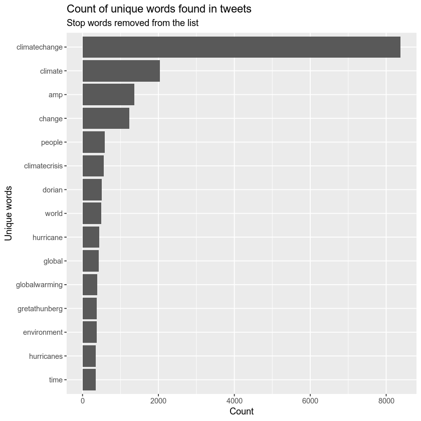
Now that you’ve performed this final step of cleaning, you can try to plot, once again.
# plot the top 15 words -- notice any issues?
cleaned_tweet_words %>%
  count(word, sort = TRUE) %>%
  top_n(15) %>%
  mutate(word = reorder(word, n)) %>%
  ggplot(aes(x = word, y = n)) +
  geom_col() +
  xlab(NULL) +
  coord_flip() +
      labs(y = "Count",
      x = "Unique words",
      title = "Count of unique words found in tweets",
      subtitle = "Stop words removed from the list")

Explore Networks of Words
You might also want to explore words that occur together in tweets. LEt’s do that next.
ngrams specifies pairs and 2 is the number of words together
# library(devtools)
#install_github("dgrtwo/widyr")
library(widyr)

# remove punctuation, convert to lowercase, add id for each tweet!
climate_tweets_paired_words <- climate_tweets %>%
  dplyr::select(stripped_text) %>%
  unnest_tokens(paired_words, stripped_text, token = "ngrams", n = 2)

climate_tweets_paired_words %>%
  count(paired_words, sort = TRUE)
## # A tibble: 134,656 x 2
##    paired_words         n
##    <chr>            <int>
##  1 climate change    1021
##  2 of the             804
##  3 in the             798
##  4 climatechange is   570
##  5 is a               442
##  6 of climatechange   437
##  7 on the             383
##  8 on climatechange   364
##  9 to the             354
## 10 this is            331
## # … with 134,646 more rows
library(tidyr)
climate_tweets_separated_words <- climate_tweets_paired_words %>%
  separate(paired_words, c("word1", "word2"), sep = " ")

climate_tweets_filtered <- climate_tweets_separated_words %>%
  filter(!word1 %in% stop_words$word) %>%
  filter(!word2 %in% stop_words$word)

# new bigram counts:
climate_words_counts <- climate_tweets_filtered %>%
  count(word1, word2, sort = TRUE)

head(climate_words_counts)
## # A tibble: 6 x 3
##   word1         word2             n
##   <chr>         <chr>         <int>
## 1 climate       change         1021
## 2 climatechange climatecrisis   232
## 3 climatechange globalwarming   147
## 4 global        warming         141
## 5 hurricane     dorian          113
## 6 climate       crisis          100
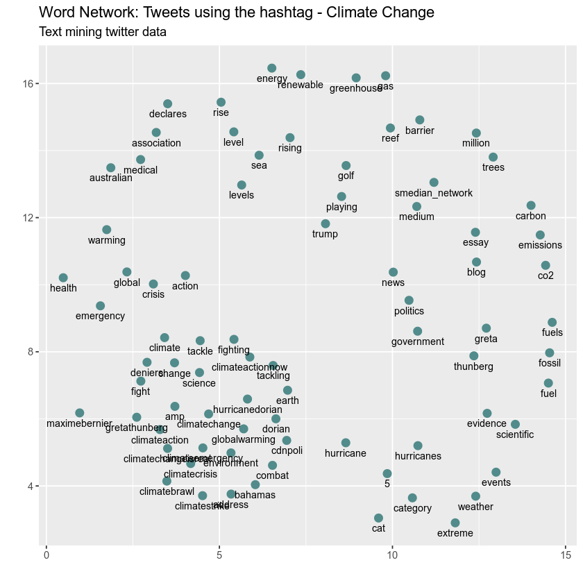
Finally, plot the data
library(igraph)
library(ggraph)

# plot climate change word network
# (plotting graph edges is currently broken)
climate_words_counts %>%
        filter(n >= 24) %>%
        graph_from_data_frame() %>%
        ggraph(layout = "fr") +
        # geom_edge_link(aes(edge_alpha = n, edge_width = n))
        # geom_edge_link(aes(edge_alpha = n, edge_width = n)) +
        geom_node_point(color = "darkslategray4", size = 3) +
        geom_node_text(aes(label = name), vjust = 1.8, size = 3) +
        labs(title = "Word Network: Tweets using the hashtag - Climate Change",
             subtitle = "Text mining twitter data ",
             x = "", y = "")

You expect the words climate & change to have a high
Share on
Twitter Facebook Google+ LinkedIn
Leave a Comment