Lesson 7. Programmatically Accessing Geospatial Data Using API’s - Working with and Mapping JSON Data from the Colorado Information Warehouse in R
Learning Objectives
After completing this tutorial, you will be able to:
- Extract geospatial (x,y) coordinate information embedded within a JSON hierarchical data structure.
- Use the
flatten()function to remove nested data.frames from data imported in JSON format. - Create a map of geospatial data using
ggmap().
What You Need
You will need a computer with internet access to complete this lesson.
In the previous lesson, you learned how to work with JSON data accessed via the Colorado information warehouse. In this lesson, you will explore another dataset; however this time, the data will contain geospatial information nested within it that will allow us to create a map of the data.
Working with Geospatial Data
Check out the map Colorado DWR Current Surface Water Conditions map. If you remember from the previous lesson, APIs can be used for many different things. Web developers (people who program and create web sites and cool applications) can use API’s to create user friendly interfaces - like the map in this link that allow us to look at and interact with data. These API’s are similar to - if not the same as the ones that you often use to access data in R.
In this lesson, you will access the data used to create the map at the link above - in R.
- The data that you will use are located here: View JSON format data used to create surface water map.
- And you can learn more about the data here: View CO Current water surface .
# load packages
library(dplyr)
library(ggplot2)
library(rjson)
library(jsonlite)
library(ggmap)
# get URL
water_base_url <- "https://data.colorado.gov/resource/j5pc-4t32.json?"
water_full_url <- paste0(water_base_url, "station_status=Active",
            "&county=BOULDER")
water_data_url <- URLencode(water_full_url)

water_data_df <- fromJSON(water_data_url)
ATTENTION WINDOWS USERS: We have noticed a bug where on windows machines, sometimes the https URL doesn’t work. Instead, try the same url as above but without the s - like this: water_base_url <- "http://data.colorado.gov/resource/j5pc-4t32.json?" This change has resolved many issues on windows machines so give it a try if you are having problems with the API.
Remember that the JSON structure supports hierarchical data and can be NESTED.
[ {
  "station_name" : "SOUTH PLATTE RIVER AT COOPER BRIDGE NEAR BALZAC",
  "amount" : "262.00",
  "flag" : "na",
  "station_status" : "Gage temporarily anavailable",
  "county" : "MORGAN",
  "wd" : "1",
  "dwr_abbrev" : "PLABALCO",
  "data_source" : "Co. Division of Water Resources",
  "http_linkage" : {
    "url" : "http://www.dwr.state.co.us/SurfaceWater/data/detail_graph.aspx?ID=PLABALCO&MTYPE=DISCHRG"
  },
  "div" : "1",
  "date_time" : "2017-02-15T09:00:00",
  "stage" : "1.86",
  "usgs_station_id" : "06759910",
  "variable" : "DISCHRG",
  "location" : {
    "latitude" : "40.357498",
    "needs_recoding" : false,
    "longitude" : "-103.528053"
  },
  "station_type" : "Stream"
}
...
]
If you look at the structure of the .json file below, you can see that the location object, is nested with three sub objects:
- latitude
- needs_recoding
- longitude
[ {
"div" : "1",
"date_time" : "2017-02-15T09:00:00",
"stage" : "1.86",
"usgs_station_id" : "06759910",
"variable" : "DISCHRG",
"location" : {
  "latitude" : "40.357498",
  "needs_recoding" : false,
  "longitude" : "-103.528053"
},
"station_type" : "Stream"
}
...
]
Next, let’s look at the structure of the data.frame that R creates from the .json data.
# view data structure
typeof(water_data_df)
## [1] "list"
In this case, you have a data.frame nested within a data.frame.
# view first 6 lines of the location nested data.frame
head(water_data_df$location)
##    latitude needs_recoding   longitude
## 1 40.211389          FALSE -105.250952
## 2  40.17708          FALSE -105.178567
## 3 40.193019          FALSE -105.210388
## 4 40.187578          FALSE -105.189191
## 5 40.153363          FALSE -105.088695
## 6 40.086278          FALSE -105.217519
# view for 6 lines of the location.latitude column
head(water_data_df$location$latitude)
## [1] "40.211389" "40.17708"  "40.193019" "40.187578" "40.153363" "40.086278"
You can remove the nesting using the flatten() function in R. When you flatten your json data, R creates new columns for each nested data.frame column. In this case it creates a unique column for latitude and longitude. Notice that the name of each new column contains the name of the previously nested data.frame followed by a period, and then the column name. For example
location.latitude
# remove the nested data frame
water_data_df <- flatten(water_data_df, recursive = TRUE)
water_data_df$location.latitude
##  [1] "40.211389" "40.17708"  "40.193019" "40.187578" "40.153363"
##  [6] "40.086278" "40.00638"  "40.17395"  "40.260827" "40.212505"
## [11] "40.091391" "39.947704" "40.177423" "40.215043" "39.938351"
## [16] "40.257844" "40.18188"  "40.258367" "40.129806" "40.07856"
## [21] "40.211083" "40.170998" "40.193758" "39.931813" "40.053035"
## [26] "40.196422" "40.204193" "40.018667" "40.220702" "40.188579"
## [31] "40.258038" "40.255776" "40.134278" "40.042028" "40.059809"
## [36] "40.172925" "40.219046" "40.09082"  "40.216263" "39.931597"
## [41] "40.185033" "40.153341" "40.199321" "39.961655" "40.126389"
## [46] "39.986169" "40.218335" "40.256276" "40.051652" "40.215658"
## [51] "40.212658" "40.19328"  "40.215904" "40.174844" "40.053661"
## [56] "40.187524" "39.931659"
Now you can clean up the data. Notice that your longitude and latitude values are in quotes. What does this mean about the structure of the data?
str(water_data_df$location.latitude)
##  chr [1:57] "40.211389" "40.17708" "40.193019" "40.187578" "40.153363" ...
In order to map or work with latitude and longitude data, you need numeric values. You can use the same dplyr function - mutate_at() - that you used in the previous lessons, to convert columns that are numbers to numeric rather than char data types:
Notice in the code below that there is an addition pipe that removes NA values (missing latitude values) from the dataset. You want to create a map of these data. You will not be able to map points with missing X,Y coordinate locations so it is best to remove them.
# where are the cells with NA values in your data?
is.na(water_data_df$location.latitude)
##  [1] FALSE FALSE FALSE FALSE FALSE FALSE FALSE FALSE FALSE FALSE FALSE
## [12] FALSE FALSE FALSE FALSE FALSE FALSE FALSE FALSE FALSE FALSE FALSE
## [23] FALSE FALSE FALSE FALSE FALSE FALSE FALSE FALSE FALSE FALSE FALSE
## [34] FALSE FALSE FALSE FALSE FALSE FALSE FALSE FALSE FALSE FALSE FALSE
## [45] FALSE FALSE FALSE FALSE FALSE FALSE FALSE FALSE FALSE FALSE FALSE
## [56] FALSE FALSE
Note, in the code above, you can identify each location where there is a NA value in your data. If you add an ! to your code, R returns the INVERSE of the above.
# where are calls with values in your data?
!is.na(water_data_df$location.latitude)
##  [1] TRUE TRUE TRUE TRUE TRUE TRUE TRUE TRUE TRUE TRUE TRUE TRUE TRUE TRUE
## [15] TRUE TRUE TRUE TRUE TRUE TRUE TRUE TRUE TRUE TRUE TRUE TRUE TRUE TRUE
## [29] TRUE TRUE TRUE TRUE TRUE TRUE TRUE TRUE TRUE TRUE TRUE TRUE TRUE TRUE
## [43] TRUE TRUE TRUE TRUE TRUE TRUE TRUE TRUE TRUE TRUE TRUE TRUE TRUE TRUE
## [57] TRUE
Thus in your dplyr pipe, the code below removes all ROWS cells with a NA value in the latitude column.
Remove NA Values: filter(!is.na(location.latitude))
# turn columns to numeric and remove NA values
water_data_df <- water_data_df %>%
  mutate_at(c( "amount", "location.longitude", "location.latitude"),
            as.numeric) %>%
  filter(!is.na(location.latitude))
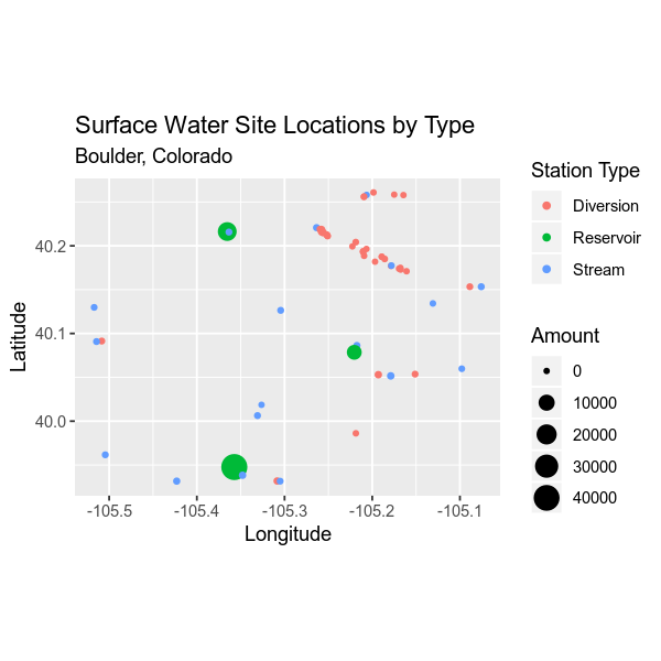
Now you can plot the data.
ggplot(water_data_df, aes(location.longitude, location.latitude, size = amount,
  color = station_type)) +
  geom_point() + coord_equal() +
      labs(x = "Longitude",
           y = "Latitude",
          title = "Surface Water Site Locations by Type",
          subtitle = "Boulder, Colorado") +
  labs(size = "Amount", colour = "Station Type")

Plotting the data using ggplot() creates a scatterplot of longitude and latitude, with some minor aesthetic tweaks. You really want to create a web map like the Colorado DWR Current Surface Water Conditions map.
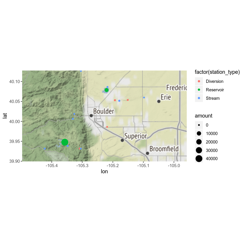
You can create a non-interactive version of this map using the ggmap() package in R. You used ggmap() earlier in the semester. It provides an efficient way to quickly draw a basemap on the fly. You can overlay your data on top of that basemap to create a nice static map.
boulder <- get_stamenmap(bbox = c(left = -105.4969, bottom = 39.8995, right =
  -104.9579, top = 40.1274), zoom = 10, messaging = FALSE, urlonly = FALSE,
  filename = NULL, color = "color")

ggmap(boulder) +
  geom_point(data = water_data_df, aes(location.longitude, location.latitude, size = amount,
  color = factor(station_type)))

In the next lesson, you will learn how to create interactive maps using the leaflet package for R.
Additional Resources
Share on
Twitter Facebook Google+ LinkedIn
Leave a Comment