Lesson 5. Programmatically Access Data Using an API in R - The Colorado Information Warehouse
Learning Objectives
After completing this tutorial, you will be able to:
- Access data from the Colorado information warehouse RESTful API.
- Describe and recognize query parameters in a RESTful call.
- Define response and request relative to data API data access.
- Define API endpoint in the context of the SODA API.
- Be able to list the 2 potential responses that you may get when querying a RESTful API.
- Use the
mutate_at()function with dplyr pipes to adjust the format / data type of multiple columns.
What You Need
You will need a computer with internet access to complete this lesson.
In the previous lessons, you learned how to access human readable text files data programmatically using:
download.file()to download a file to your computer and work with it (ideal if you want to save a copy of the data to your computer)read.csv()ideal for reading in a tabular file stored on the web but may sometimes fail when there are secure connections involved (e.g. https).fromJSON()ideal for data accessed in JSON format.
In this lesson, you will learn about API interfaces. An API allows us to access data stored on a computer or server using a specific query. APIs are powerful ways to access data and more specifically the specific type and subset of data that you need for your analysis, programmatically.
You will also explore the machine readable JSON data structure. Machine readable data structures are more efficient - particularly for larger data that contain hierarchical structures. In this lesson, you will use the getJSON() function from the rjson package to import data from an API, provided in .json format into a data.frame.
#NOTE: if you have problems with ggmap, try to install both ggplot and ggmap from github
#devtools::install_github("dkahle/ggmap")
#devtools::install_github("hadley/ggplot2")
library(ggmap)
library(ggplot2)
library(dplyr)
library(rjson)
library(jsonlite)
library(RCurl)
REST API Review
Remember that in the first lesson in this module, you learned about RESTful APIs. You explored the concept of a request and then a subsequent response. The request to an RESTful API is composed of a URL and the associated parameters required to access a particular subset of the data that you wish to access.
When you send the request, the web API returns one of the following:
- The data that you requested or
- A failed to return message which tells us that something was wrong with your request.
In this lesson you will access data stored in JSON format from a RESTful API.
Colorado Population Projection data
The Colorado Information Marketplace is a comprehensive data warehouse that contains a wide range of Colorado-specific open datasets available via a RESTful API called the Socrata Open Data API (SODA).
API Endpoints
There are lots of API endpoints or data sets available via this API. An endpoint refers to a dataset that you can access and query against.
The “endpoint” of a (SODA) API is simply a unique URL that represents an object or collection of objects. Every Socrata dataset, and even every individual data record, has its own endpoint. The endpoint is what you’ll point your HTTP client at to interact with data resources. Read more about endpoints
One endpoint on the CO information warehouse website contains Colorado Population Projections. If you click on the Colorado Population Projections data link (JSON format) you will see data returned in a JSON format. These data include population estimates for males and females for every county in Colorado for every year from 1990 to 2040 for multiple age groups.
URL Parameters
Using URL parameters, you can define a more specific request to limit what data you get back in response to your API request. For example, if you only want data for Boulder, Colorado, you can query just that subset of the data using the RESTful call. In the link below, note that the ?&county=Boulder part of the url makes the request to the API to only return data that are for Boulder County, Colorado.
Like this: https://data.colorado.gov/resource/tv8u-hswn.json?&county=Boulder.
Parameters associated with accessing data using this API are documented here.
Using the Colorado SODA API
The Colorado SODA API allows us to write ‘queries’ that filter out the exact subset of the data that you want. Here’s the API URL for population projections for females who live in Boulder that are age 20-40 for the years 2016-2025:
https://data.colorado.gov/resource/tv8u-hswn.json?$where=age between 20 and 40 and year between 2016 and 2025&county=Boulder&$select=year,age,femalepopulation
Click here to view data. (JSON format).
API Response
The data that are returned from an API request are called the response. The format of the returned data or the response is most often in the form of plain text ‘file’ such as JSON or .csv.
Data Tip: Many API’s allow us to specify the format of the data that you want returned in the response. The Colorado SODA API is no exception - check out the documentation.
Accessing API Data
The first thing that you need to do is create your API request string. Remember that this is a URL with parameters parameters that specify which subset of the data that you want to access.
Note that you are using a new function - paste0() - to paste together a complex URL string. This is useful because you may want to iterate over different subsets of the same data (ie reuse the base url or the endpoint but request different subsets using different URL parameters).
# Base URL path
base_url = "https://data.colorado.gov/resource/tv8u-hswn.json?"
full_url = paste0(base_url, "county=Boulder",
             "&$where=age between 20 and 40",
             "&$select=year,age,femalepopulation")

# view full url
full_url
## [1] "https://data.colorado.gov/resource/tv8u-hswn.json?county=Boulder&$where=age between 20 and 40&$select=year,age,femalepopulation"
After you’ve created the URL, you can get the data. There are a few ways to access the data however the most direct way is to
- Use
encodeURL()to replace spaces in your url with the asii value for space%20 - Use the
fromJSON()function in the rjson package to import that data into a data.frame object.
Let’s give it a try. First, you encode the URL to replace all spaces with the ascii value for a space which is %20.
# encode the URL with characters for each space.
full_url <- URLencode(full_url)
full_url
## [1] "https://data.colorado.gov/resource/tv8u-hswn.json?county=Boulder&$where=age%20between%2020%20and%2040&$select=year,age,femalepopulation"
Then, you import the data directly into a data.frame using the fromJSON() function that is in the rjson package.
library(rjson)

# Convert JSON to data frame
pop_proj_data_df <- fromJSON(getURL(full_url))
head(pop_proj_data_df, n = 2)
##   year age femalepopulation
## 1 1990  20             2751
## 2 1990  21             2615
typeof(pop_proj_data_df)
## [1] "list"
Data Tip: The getForm() is another way to access API driven data. You are not going to learn this in this class however it is a good option that results in code that is a bit cleaner given the various parameters are passed to the function via argument like syntax.
base_url_example <- "https://data.colorado.gov/resource/tv8u-hswn.json?"
getForm(base_url, county = "Boulder",
             age="BOULDER")
Also note that if you wanted to use getURL(), you could do so as follows:
# get the data from the specified url using RCurl
pop_proj_data_example <- getURL(URLencode(full_url))
Now that your data are in a data.frame format, you can clean them up. Let’s have a close look at the data structure. Are the values in the correct format to work with them quantitatively?
# view data structure
str(pop_proj_data_df)
## 'data.frame':	1000 obs. of  3 variables:
##  $ year            : chr  "1990" "1990" "1990" "1990" ...
##  $ age             : chr  "20" "21" "22" "23" ...
##  $ femalepopulation: chr  "2751" "2615" "2167" "1798" ...
When you import the data from JSON, by default they import in string format. However, if you want to plot the data and manipulate the data quantitatively, you need your data to be in a numeric format. Let’s fix that next.
mutate_at from dplyr
You can uset the mutate_at() function in a dplyr pipe to change the format of (or apply any function on) any columns within your data.frame. In this case you want to convert all of the columns to a numeric format.
To use mutate_at() you specify the column names that you want to convert in a vector followed by the function that you wish to apply to each column. THe function in this case is as.numeric().
Because you are using this function in a pipe, your code looks like this:
# turn columns to numeric and remove NA values
pop_proj_data_df <- pop_proj_data_df %>%
 mutate_at(c( "age", "year", "femalepopulation"), as.numeric)

str(pop_proj_data_df)
## 'data.frame':	1000 obs. of  3 variables:
##  $ year            : num  1990 1990 1990 1990 1990 1990 1990 1990 1990 1990 ...
##  $ age             : num  20 21 22 23 24 25 26 27 28 29 ...
##  $ femalepopulation: num  2751 2615 2167 1798 1692 ...
Data Tip: Note that the code below, is much more VERBOSE version of what you did above, in a clean way using mutate_at(). dplyr is a much more efficient way to convert the format of several columns of information!
# convert EACH row to a numeric format
# note this is the clunky way to do what you did above with dplyr!
pop_proj_data_df$age <- as.numeric(pop_proj_data_df$age)
pop_proj_data_df$year <- as.numeric(pop_proj_data_df$year)
pop_proj_data_df$femalepopulation <- as.numeric(pop_proj_data_df$femalepopulation)

# OR use the apply function to convert all rows in the data.frame to numbers
#pops <- as.data.frame(lapply(pop_proj_data_df, as.numeric))
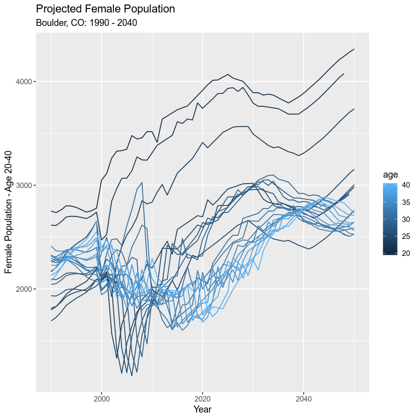
Once you have converted your data to a numeric format, you can plot it using ggplot().
# plot the data
ggplot(pop_proj_data_df, aes(x = year, y = femalepopulation,
 group = factor(age), color = age)) + geom_line() +
     labs(x = "Year",
          y = "Female Population - Age 20-40",
          title = "Projected Female Population",
          subtitle = "Boulder, CO: 1990 - 2040")

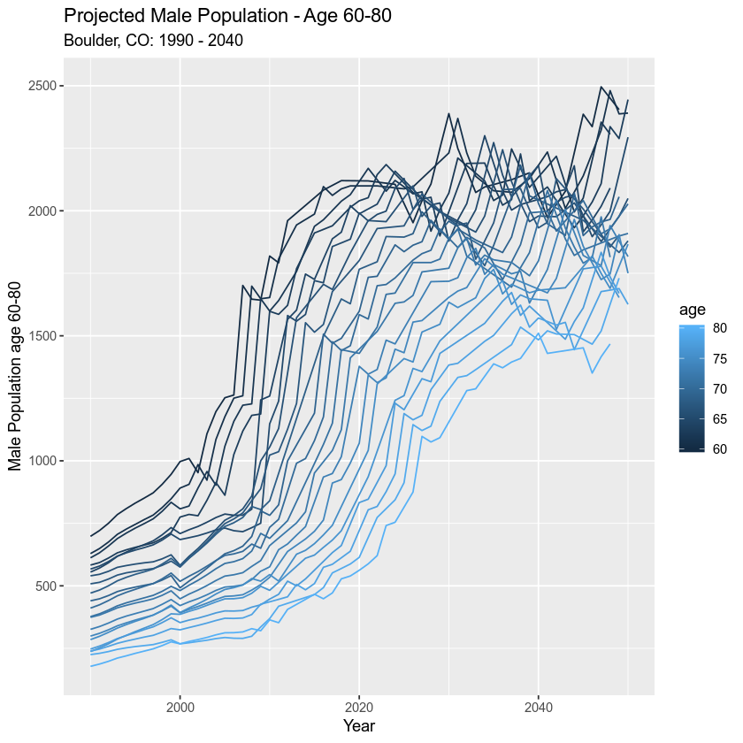
Optional Challenge
Using the population projection data that you just used, create a plot of projected MALE population numbers as follows:
- Time span: 1990-2040
- Column category: malepopulation
- Age range: 60-80 years old
Use ggplot() to create your plot and be sure to label x and y axes and give the plot a descriptive title.
Example Homework Plot

Additional Resources
Share on
Twitter Facebook Google+ LinkedIn
Leave a Comment