In the previous tutorials we’ve learned about the R Markdown format and how to create a report using R Markdown in RStudio. In this tutorial, we will render or knit an R Markdown document to a web friendly, html format using the R knitr package. knitr can be used to convert R Markdown files to many different formats including: html, pdf, GitHub markdown (.md) and more.

What is Knitr?

knitr is the R package that we use to convert an R Markdown document into another, more user friendly format like .html or .pdf.

The knitr package allows us to:

• Publish & share preliminary results with collaborators.
• Create professional reports that document our workflow and results directly from our code, reducing the risk of accidental copy and paste or transcription errors.
• Document our workflow to facilitate reproducibility.
• Efficiently change code outputs (figures, files) given changes in the data, methods, etc.

The knitr package was designed to be a transparent engine for dynamic report generation with R – Yihui Xi – knitr package creator

When To Knit: Knitting is a useful exercise throughout your scientific workflow. It allows you to see what your outputs look like and also to test that your code runs without errors. The time required to knit depends on the length and complexity of the script and the size of your data.

How to Knit

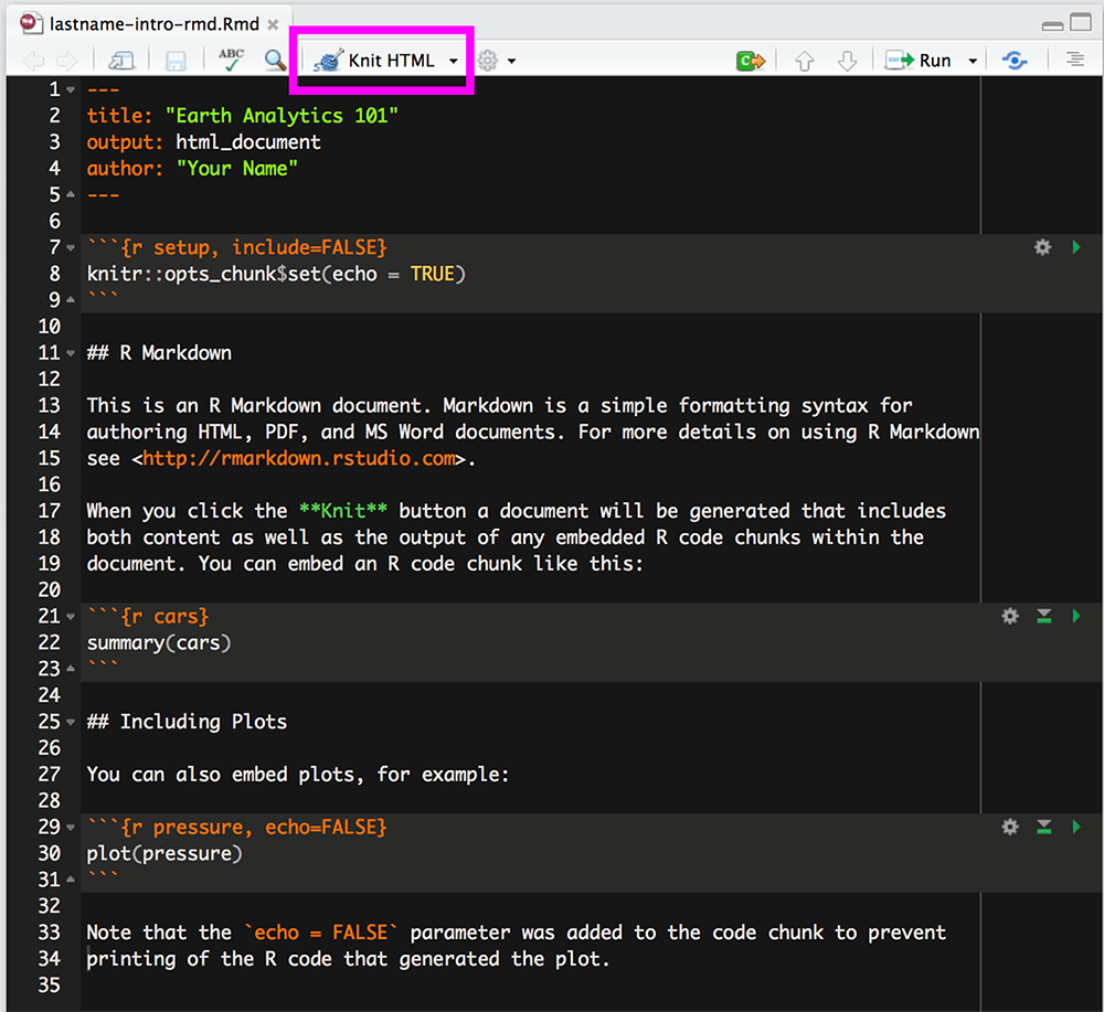
To knit in RStudio, click the Knit pull down button. You want to use the Knit HTML option for this lesson.

When you click the Knit HTML button, a window will open in your console titled R Markdown. This pane shows the knitting progress. The output (html in this case) file will automatically be saved in the current working directory. If there is an error in the code, an error message will appear with a line number in the R Console to help you diagnose the problem.

Data tip: You can run knitr from the command prompt using: render(“input.Rmd”, “all”).

View the Output

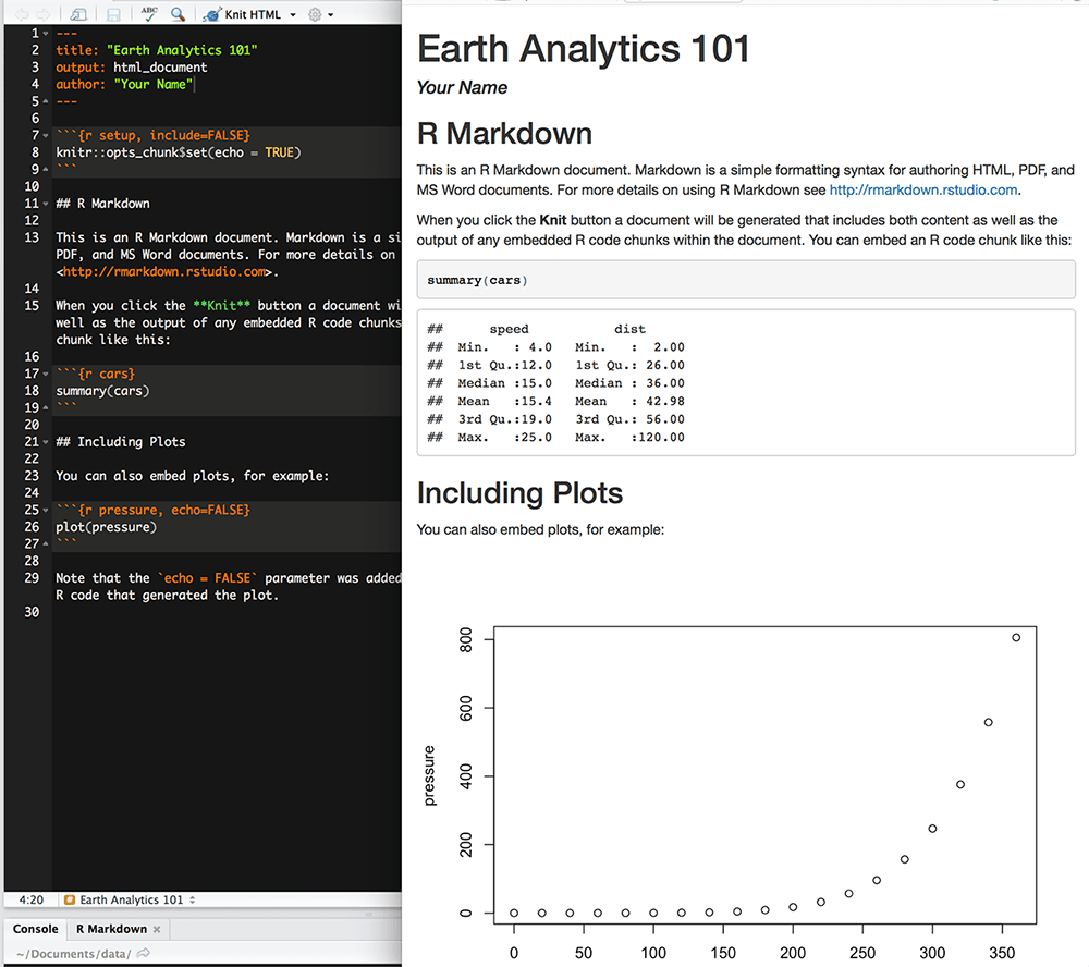
When knitting is complete, the html file produced will automatically open.

Notice that information from the YAML header (title, author, date) is printed at the top of the HTML document. Then the html shows the text, code, and results of the code that you included in the Rmd document.

# load the ggplot2 library for plotting
library(ggplot2)

# download data from figshare
# note that we are downloading  the data into your working directory (earth-analytics)
download.file(url = "https://ndownloader.figshare.com/files/7010681",
              destfile = "data/boulder-precip.csv")

# import data
boulder_precip <- read.csv(file="data/boulder-precip.csv")

# view first few rows of the data
head(boulder_precip)

# when we download the data we create a dataframe
# view each column of the data frame using it's name (or header)
boulder_precip$DATE

# view the precip column
boulder_precip$PRECIP

# q plot stands for quick plot. Let's use it to plot our data
qplot(x=boulder_precip$DATE,
      y=boulder_precip$PRECIP)

When you knit your .Rmd file to pdf, the plot you produce should look like the one below. Not so pretty, eh? Don’t worry - we will learn more about plotting in a later tutorial!

Where is the File?

In the steps above, we downloaded a file. However, where did that file go on your computer? Let’s find it before we go any further.

# what is the working directory?
getwd()

[1] "/Users/lewa8222/Documents/earth-analytics"

# set working dir as a variable
my.dir <- getwd()

# what files are in that working directory?
list.files(my.dir, recursive= TRUE)

Is the boulder-precip.csv file there?