Lesson 6. Test Your Skills: Open Raster Data Using RioXarray In Open Source Python
Learning Objectives
- Practice your skills manipulating raster data using rioxarray.
# Import necessary packages
import os
import matplotlib.pyplot as plt
import seaborn as sns
import geopandas as gpd
import rioxarray as rxr
# Plotting extent is used to plot raster & vector data together
from rasterio.plot import plotting_extent

import earthpy as et
import earthpy.plot as ep

# Prettier plotting with seaborn
sns.set(font_scale=1.5, style="white")
# Get data and set working directory
et.data.get_data("colorado-flood")
os.chdir(os.path.join(et.io.HOME, 'earth-analytics', 'data'))
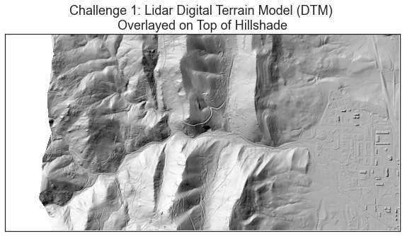
Challenge 1: Open And Plot Hillshade
It’s time to practice your raster skills. Do the following:
Use the pre_DTM_hill.tif layer in the colorado-flood/spatial/boulder-leehill-rd/pre-flood/lidar directory.
- Open the
pre_DTM_hill.tiflayer using rioxarray. - Plot the data using
ep.plot_bands(). - Set the colormap (
cmap=) parameter value to Greys:cmap="gray"
Give you plot a title.
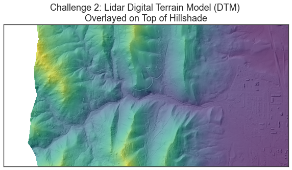
Challenge 2: Overlay DTM Over DTM Hillshade
In the challenge above, you opened and plotted a hillshade of the lidar digital terrain model create from NEON lidar data before the 2013 Colorado Flood. In this challenge, you will use the hillshade to create a map that looks more 3-dimensional by overlaying the DTM data on top of the hillshade.
To do this, you will need to plot each layer using ep.plot_bands()
- Plot the hillshade layer
pre_DTM_hill.tifthat you opened in Challenge 1. Similar to Challenge one setcmap="gray" - Plot the DTM that you opened above
dtm_pre_arr- When you plot the DTM, use the
alpha=parameter to adjust the opacity of the DTM so that you can see the shading on the hillshade underneath the DTM. - Set the colormap to viridis (or any colormap that you prefer)
cmap='viridis'for the DTM layer.
- When you plot the DTM, use the
HINT: be sure to use the ax= parameter to make sure both layers are on the same figure.
Data Tip:
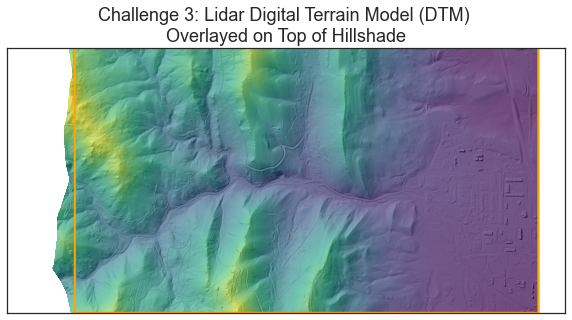
Challenge 3: Add A Site Boundary to Your Raster Plot
Take all of the code that you wrote above to plot the DTM on top of your hillshade layer. Add the site boundary layer that you opened above site_bound_shp to your plot.
HINT: remember that the plotting_extent() object (lidar_dem_plot_ext) will be needed to add this final layer to your plot.
Data Tip: Plotting Raster and Vector Together
You can learn more about overlaying vector data on top of raster data to create maps in Python in this lesson on setting plotting extents.
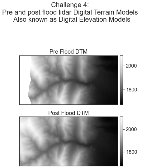
Challenge 4 (Optional): Open Post Flood Raster
Above, you opened up a lidar derived Digital Terrain Model (DTM or DEM) that was created from data collected before the 2013 flood. In the post-flood directory, you will find a DTM containing data collected after the 2013 flood.
Create a figure with two plots.
In the first subplot, plot the pre-flood data that you opened above. In the second subplot, open and plot the post-flood DTM data. You wil find the file post_DTM.tif in the post-flood directory of your colorado-flood dataset downloaded using earthpy.
- Add a super title (a title for the entire figure) using
plt.suptitle("Title Here") - Adjust the location of your suptitle
plt.tight_layout(rect=[0, 0.03, 1, 0.9])
Share on
Twitter Facebook Google+ LinkedIn