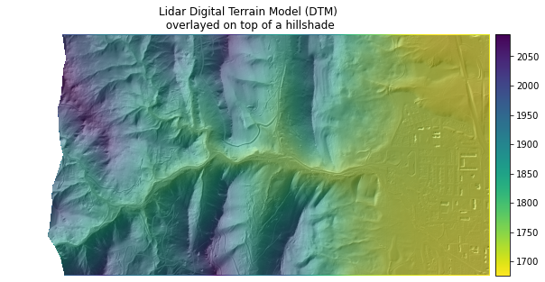
Lesson 2. Layer a raster dataset over a hillshade in Python to create a beautiful basemap that represents topography.
Learning Objectives
- Overlay two rasters in Python to create a plot.
Overlay Rasters in Python
In this lesson, you will learn about overlaying rasters on top of a hillshade for nicer looking plots in Python.
To overlay a raster, you will plot two different raster datasets in the same plot in matplotlib such as a Digital Terrain Model (DTM) and a hillshade raster.
You will use the alpha parameter of ep.plot_bands to adjust the transparency of rasters, so that the terrain hillshade gives the DTM raster texture! You will also turn off the legend for the hillshade, as the legend you want to see is the DTM elevation values.
What is a Hillshade?
A hillshade is a representation of the earth’s surface as it would look with shade and shadows from the sun. You often render a hillshade using a greyscale colorramp.
Hillshades make nice underlays for other data as they emphasize the topography visually. This adds depth to your map!
To begin, open up both the Digital Terrain Model (DTM) and the DTM hillshade files.
import os
import matplotlib.pyplot as plt
import numpy as np
import rioxarray as rxr
import earthpy as et
import earthpy.plot as ep

# Import data from EarthPy
data = et.data.get_data('colorado-flood')

# Set working directory
os.chdir(os.path.join(et.io.HOME, 'earth-analytics', 'data'))
Downloading from https://ndownloader.figshare.com/files/16371473
Extracted output to /root/earth-analytics/data/colorado-flood/.
# Open DTM data
lidar_dem_path = os.path.join("colorado-flood",
                              "spatial",
                              "boulder-leehill-rd",
                              "pre-flood",
                              "lidar",
                              "pre_DTM.tif")

lidar_dem_im = rxr.open_rasterio(lidar_dem_path, masked=True)

# Open DTM hillshade
lidar_hs_path = os.path.join("colorado-flood",
                             "spatial",
                              "boulder-leehill-rd",
                             "pre-flood",
                              "lidar",
                             "pre_DTM_hill.tif")

lidar_dem_hill = rxr.open_rasterio(lidar_hs_path, masked=True)
To plot both layers together, you use the same ax object for the two layers, and then add a alpha value to the DTM hillshade image. This value makes the image more transparent.
Below an alpha of 0.5 (50%) is applied. Play around with the alpha value to see how it impacts your map.
fig, ax = plt.subplots(figsize=(10, 6))

ep.plot_bands(lidar_dem_im,
              ax=ax,
              cmap='viridis_r',
              title="Lidar Digital Terrain Model (DTM)\n overlayed on top of a hillshade")

ep.plot_bands(lidar_dem_hill,
              cmap='Greys',
              alpha=0.5,
              ax=ax,
              cbar=False)

ax.set_axis_off()

plt.show()

Share on
Twitter Facebook Google+ LinkedIn
Leave a Comment