Lesson 1. Introduction to Multispectral Remote Sensing Data in Python
Learn How to Work With Multispectral Remote Sensing Data in Python - Intermediate earth data science textbook course module
Welcome to the first lesson in the Learn How to Work With Multispectral Remote Sensing Data in Python module. Learn how to use spectral remote sensing data to better understand fire activity.Chapter Seven - Intro to Multispectral Remote Sensing Data
In this chapter, you will learn about various options for multispectral remote sensing data and the advantages and disadvantages of these data options.
Learning Objectives
After completing this chapter, you will be able to:
- Define spectral and spatial resolution and explain how they differ from one another.
- Define multispectral (or multi-band) remote sensing data.
- Describe at least 3 differences between NAIP imagery, Landsat 8 and MODIS in terms of how the data are collected, how frequently they are collected and the spatial and spectral resolution.
- Describe the spatial and temporal tradeoffs between data collected from a satellite vs an airplane.
What You Need
You will need a computer with internet access to complete this chapter.
About Spectral Remote Sensing
In the previous weeks of this course, you learned about lidar remote sensing. If you recall, a lidar instrument is an active remote sensing instrument. This means that the instrument emits energy actively rather than collecting information about light energy from another source (the sun). This week you will work with multispectral imagery or multispectral remote sensing data. Multispectral remote sensing is a passive remote sensing type. This means that the sensor is measuring light energy from an existing source - in this case the sun.


Electromagnetic Spectrum
To better understand multispectral remote sensing you need to know some basic principles of the electromagnetic spectrum.
The electromagnetic spectrum is composed of a range of different wavelengths or “colors” of light energy. A spectral remote sensing instrument collects light energy within specific regions of the electromagnetic spectrum. Each region in the spectrum is referred to as a band.
Above: A video overview of spectral remote sensing.
Above: Watch the first 8 minutes for a nice overview of spectral remote sensing.
Key Attributes of Spectral Remote Sensing Data
Space vs Airborne Data
Remote sensing data can be collected from the ground, the air (using airplanes or helicopters) or from space. You can imagine that data that are collected from space are often of a lower spatial resolution than data collected from an airplane. The tradeoff however is that data collected from a satellite often offers better (up to global) coverage.
For example the Landsat 8 satellite has a 16 day repeat cycle for the entire globe. This means that you can find a new image for an area, every 16 days. It takes a lot of time and financial resources to collect airborne data. Thus data are often only available for smaller geographic areas. Also, you may not find that the data are available for the time periods that you need. For example, in the case of NAIP, you may only have a new dataset every 2-4 years.

Bands and Wavelengths
When talking about spectral data, you need to understand both the electromagnetic spectrum and image bands. Spectral remote sensing data are collected by powerful camera-like instruments known as imaging spectrometers. Imaging spectrometers collect reflected light energy in “bands.”
A band represents a segment of the electromagnetic spectrum. You can think of it as a bin of one “type” of light. For example, the wavelength values between 800 nanometers (nm) and 850 nm might be one band captured by an imaging spectrometer. The imaging spectrometer collects reflected light energy within a pixel area on the ground. Since an imaging spectrometer collects many different types of light - for each pixel the amount of light energy for each type of light or band will be recorded. So, for example, a camera records the amount of red, green and blue light for each pixel.
Often when you work with a multispectral dataset, the band information is reported as the center wavelength value. This value represents the center point value of the wavelengths represented in that band. Thus in a band spanning 800-850 nm, the center would be 825 nm.

Spectral Resolution
The spectral resolution of a dataset that has more than one band, refers to the spectral width of each band in the dataset. In the image above, a band was defined as spanning 800-810 nm. The spectral width or spectral resolution of the band is thus 10 nm. To see an example of this, check out the band widths for the Landsat sensors.
While a general spectral resolution of the sensor is often provided, not all sensors collect information within bands of uniform widths.
Spatial Resolution
The spatial resolution of a raster represents the area on the ground that each pixel covers. If you have smaller pixels in a raster the data will appear more “detailed.” If you have large pixels in a raster, the data will appear more coarse or “fuzzy.”
If high resolution data shows you more about what is happening on the Earth’s surface why wouldn’t you always just collect high resolution data (smaller pixels)?
If you recall, you learned about raster spatial resolution when you worked with lidar elevation data in previous lessons. The same resolution concepts apply to multispectral data.

What is Multispectral Imagery?
Introduction to Multi-Band Raster Data
Earlier in this course, you worked with raster data derived from lidar remote sensing instruments. These rasters consisted of one layer or band and contained height values derived from lidar data. In this lesson, you will learn how to work with rasters containing multispectral imagery data stored within multiple bands (or layers).
Just like you did with single band rasters, you will use the rasterio.open() function to open multi band raster data in Python.
- To import multi-band raster data you will use the
stack()function. - If your multi-band data are imagery that you wish to composite into a color image, you can use the
earthpyplot_rgb()function to plot a 3 band raster image.

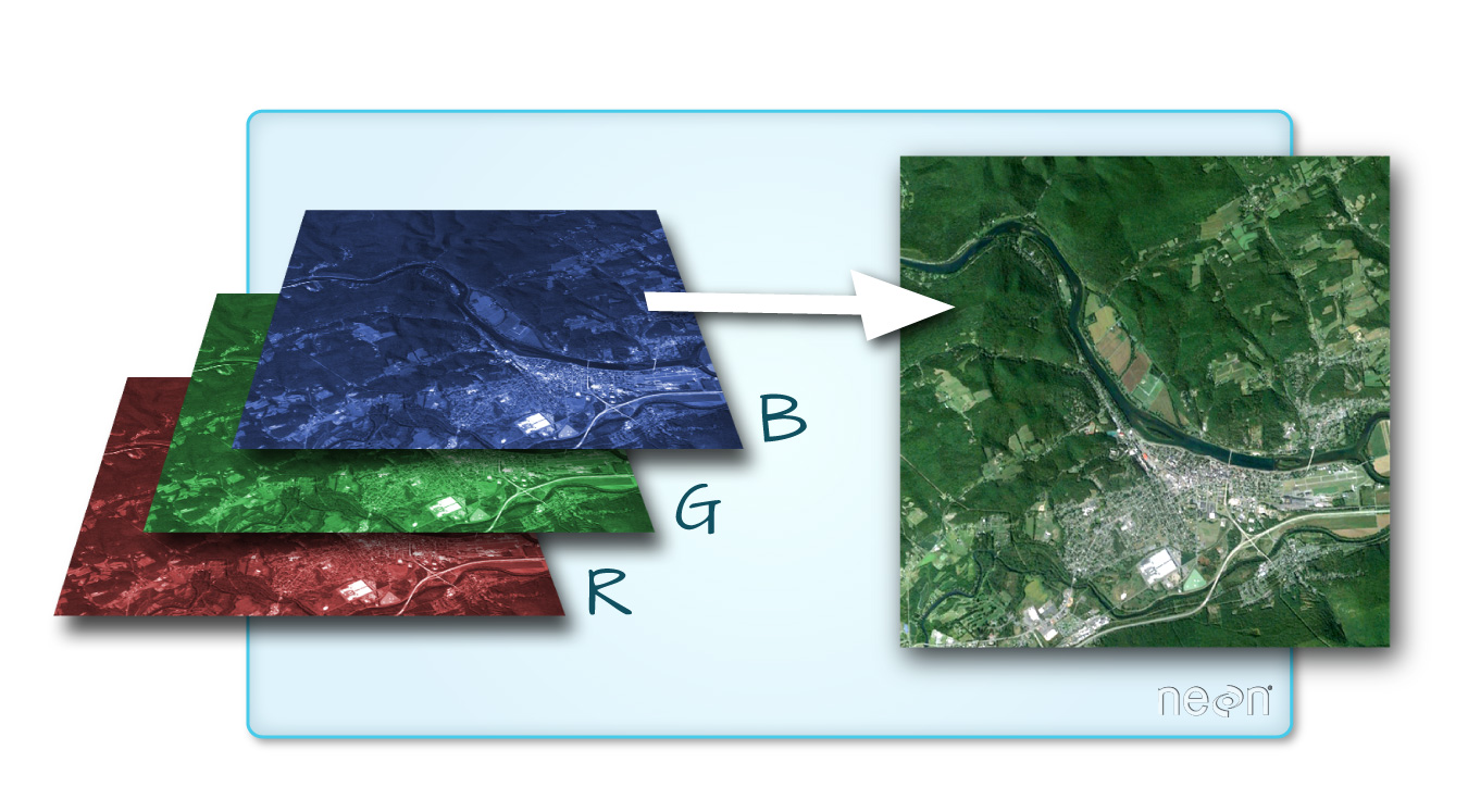
One type of multispectral imagery that is familiar to many of us is a color image. A color image consists of three bands: red, green, and blue. Each band represents light reflected from the red, green or blue portions of the electromagnetic spectrum. The pixel brightness for each band, when composited creates the colors that you see in an image. These colors are the ones your eyes can see within the visible portion of the electromagnetic spectrum.
You can plot each band of a multi-band image individually using a grayscale color gradient. Remember from the videos that you watched in class that the LIGHTER colors represent a stronger reflection in that band. DARKER colors represent a weaker reflection.

RBG Plot
You can plot the red, green and blue bands together to create an RGB image. This is what you would see with our eyes if you were in the airplane looking down at the earth.

Each band plotted separately
Note there are four bands below. You are looking at the red, green, blue and near infrared bands of a NAIP image. What do you notice about the relative darkness / lightness of each image? Is one image brighter than the other?

Color Infrared (CIR) Image
If the image has a 4th NIR band, you can create a CIR (sometimes called false color) image. In a color infrared image, the NIR band is plotted on the “red” band. Thus vegetation, which reflects strongly in the NIR part of the spectrum, is colored “red”. CIR images are often used to better understand vegetation cover and health in an area.

Other Types of Multi-band Raster Data
Multi-band raster data might also contain:
- Time series: the same variable, over the same area, over time.
- Multi or hyperspectral imagery: image rasters that have 4 or more (multi-spectral) or more than 10-15 (hyperspectral) bands.
Recall that you have worked with time series data in earlier chapters of this textbook.
NAIP, Landsat & MODIS
To begin working with multispectral remote sensing data, you will look at 2 sources of data:
- NAIP: National Agricultural Imagery Program data
- Landsat: Landuse Satellite
Later in the textbook, you will also work with MODIS (Moderate Imaging Spectrometer) data.
About NAIP Multispectral Imagery
NAIP imagery is available in the United States and typically has three bands - red, green and blue. However, sometimes, there is a 4th near-infrared band available. NAIP imagery typically is 1m spatial resolution, meaning that each pixel represents 1 meter on the Earth’s surface. NAIP data is often collected using a camera mounted on an airplane and is collected for a given geographic area every few years.
Landsat 8 Imagery
Compared to NAIP, Landsat data are collected using an instrument mounted on a satellite which orbits the globe, continuously collecting images. The Landsat instrument collects data at 30 meter spatial resolution but also has 11 bands distributed across the electromagnetic spectrum compared to the 3 or 4 that NAIP imagery has. Landsat also has one panchromatic band that collects information across the visible portion of the spectrum at 15 m spatial resolution.
Landsat 8 bands 1-9 are listed below:
Landsat 8 Bands
| Band | Wavelength range (nm) | Spatial Resolution (m) | Spectral Width (nm) |
|---|---|---|---|
| Band 1 - Coastal aerosol | 430 - 450 | 30 | 2.0 |
| Band 2 - Blue | 450 - 510 | 30 | 6.0 |
| Band 3 - Green | 530 - 590 | 30 | 6.0 |
| Band 4 - Red | 640 - 670 | 30 | 0.03 |
| Band 5 - Near Infrared (NIR) | 850 - 880 | 30 | 3.0 |
| Band 6 - SWIR 1 | 1570 - 1650 | 30 | 8.0 |
| Band 7 - SWIR 2 | 2110 - 2290 | 30 | 18 |
| Band 8 - Panchromatic | 500 - 680 | 15 | 18 |
| Band 9 - Cirrus | 1360 - 1380 | 30 | 2.0 |
Source: USGS Landsat

MODIS Imagery
The Moderate Resolution Imaging Spectrometer (MODIS) instrument is another satellite based instrument that continuously collects data over the Earth’s surface. MODIS collects spectral information at several spatial resolutions including 250m, 500m and 1000m. You will be working with the 500 m spatial resolution MODIS data in this class. MODIS has 36 bands however in class you will learn about only the first 7 bands.
First 7 MODIS Bands
Below, you can see the first 7 bands of the MODIS instrument
| Band | Wavelength range (nm) | Spatial Resolution (m) | Spectral Width (nm) | |
|---|---|---|---|---|
| Band 1 - red | 620 - 670 | 250 | 2.0 | |
| Band 2 - near infrared | 841 - 876 | 250 | 6.0 | |
| Band 3 - blue/green | 459 - 479 | 500 | 6.0 | |
| Band 4 - green | 545 - 565 | 500 | 3.0 | |
| Band 5 - near infrared | 1230 | 1250 | 500 | 8.0 |
| Band 6 - mid-infrared | 1628 | 1652 | 500 | 18 |
| Band 7 - mid-infrared | 2105 - 2155 | 500 | 18 |
Additional Resources:
Share on
Twitter Facebook Google+ LinkedIn
Leave a Comment