Lesson 2. Customize your Maps in Python: GIS in Python
Learning Objectives
After completing this tutorial, you will be able to:
- Clip a spatial vector point and line layer to the spatial extent of a polygon layer in
Python - Visually “clip” or zoom in to a particular spatial extent in a plot.
What You Need
You will need a computer with internet access to complete this lesson and the spatial-vector-lidar data subset created for the course.
Download Spatial Lidar Teaching Data Subset data
or using the earthpy package: et.data.get_data("spatial-vector-lidar")
In this lesson, you will learn how to spatially clip data for easier plotting and analysis of smaller spatial areas. You will use the geopandas library and the box module from the shapely library.
# Import libraries
import os
import numpy as np
import matplotlib.pyplot as plt
import geopandas as gpd
import earthpy as et

# Get the data
data = et.data.get_data('spatial-vector-lidar')

os.chdir(os.path.join(et.io.HOME, 'earth-analytics', 'data'))
Downloading from https://ndownloader.figshare.com/files/12459464
Extracted output to /root/earth-analytics/data/spatial-vector-lidar/.
# Read in necessary files
sjer_aoi = gpd.read_file(os.path.join("spatial-vector-lidar",
                                      "california",
                                      "neon-sjer-site",
                                      "vector_data",
                                      "SJER_crop.shp"))
country_boundary_us = gpd.read_file(os.path.join("spatial-vector-lidar",
                                                 "usa",
                                                 "usa-boundary-dissolved.shp"))
ne_roads = gpd.read_file(os.path.join("spatial-vector-lidar",
                                      "global",
                                      "ne_10m_roads",
                                      "ne_10m_n_america_roads.shp"))
Change the Spatial Extent of a Plot in Python
Above you modified your data by clipping it. This is useful when you want to
- Make your data smaller to speed up processing and reduce file size
- Make analysis simpler and faster given less data to work with.
However, if you just want to plot the data, you can consider adjusting the spatial extent of a plot to “zoom in”. Note that zooming in on a plot does not change your data in any way - it just changes how your plot renders!
To zoom in on a region of your plot, you first need to grab the spatial extent of the object
# Get spatial extent  - to zoom in on the map rather than clipping
aoi_bounds = sjer_aoi.geometry.total_bounds
aoi_bounds
array([ 254570.567     , 4107303.07684455,  258867.40933092,
       4112361.92026107])
The total_bounds attribute represents the total spatial extent for the aoi layer. This is the total external boundary of the layer - thus if there are multiple polygons in the layer it will take the furtherst edge in the north, south, east and west directions to create the spatial extent box.
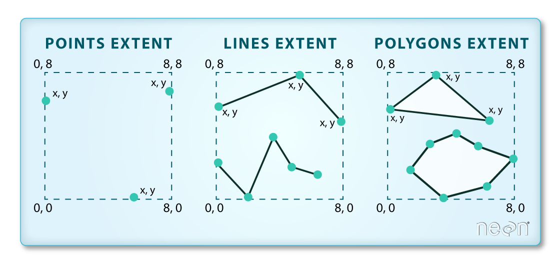
The object that is returned is a tuple - a non editable object containing 4 values: (xmin, ymin, xmax, ymax). If you want you can assign each value to a new variable as follows
# Create x and y min and max objects to use in the plot boundaries
xmin, ymin, xmax, ymax = aoi_bounds
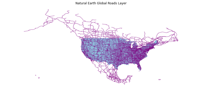
fig, ax = plt.subplots(figsize  = (14, 6))
country_boundary_us.plot(alpha = .5, ax = ax)
ne_roads.plot(color='purple', ax=ax, alpha=.5)
ax.set(title='Natural Earth Global Roads Layer')
ax.set_axis_off()
plt.axis('equal')
plt.show()
You can set the x and ylimits of the plot using the x and y min and max values from your bounds object that you created above to zoom in your map.
# Use the country boundary to set the min and max values for the plot
country_boundary_us.total_bounds
array([-124.725839, 24.498131, -66.949895, 49.384358])
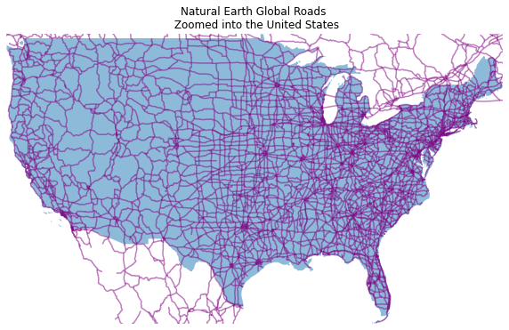
Notice in the plot below, you can still see roads that fall outside of the US Boundary area but are within the rectangular spatial extent of the boundary layer. Hopefully this helps you better understand the difference between clipping the data to a polygon shape vs simply plotting a small geographic region.
# Plot the data with a modified spatial extent
fig, ax = plt.subplots(figsize = (10,6))
xlim = ([country_boundary_us.total_bounds[0],  country_boundary_us.total_bounds[2]])
ylim = ([country_boundary_us.total_bounds[1],  country_boundary_us.total_bounds[3]])

ax.set_xlim(xlim)
ax.set_ylim(ylim)

country_boundary_us.plot(alpha = .5, ax = ax)
ne_roads.plot(color='purple', ax=ax, alpha=.5)

ax.set(title='Natural Earth Global Roads \n Zoomed into the United States')
ax.set_axis_off()
plt.show()
Share on
Twitter Facebook Google+ LinkedIn
Leave a Comment