Lesson 2. Work With Datetime Format in Python - Time Series Data
Learning Objectives
After completing this chapter, you will be able to:
- Import a time series dataset using pandas with dates converted to a
datetimeobject in Python. - Use the
datetimeobject to create easier-to-read time series plots and work with data across various timeframes (e.g. daily, monthly, yearly) in Python. - Explain the role of “no data” values and how the
NaNvalue is used in Python to label “no data” values. - Set a “no data” value for a file when you import it into a pandas dataframe.
Dive Deeper Into Working With Datetime Objects in Python
On this page, you will learn how to handle dates using the datetime object in Python with pandas, using a dataset of daily temperature (maximum in Fahrenheit) and total precipitation (inches) in July 2018 for Boulder, CO, provided by the National Oceanic and Atmospheric Administration (NOAA).
Import Packages and Get Data
To begin, import the necessary packages to work with pandas dataframe and download data. You will work with modules from pandas and matplotlib to plot dates more efficiently, and you will work with the seaborn package to make more attractive plots.
# Import necessary packages
import os
import matplotlib.pyplot as plt
import seaborn as sns
import pandas as pd
import earthpy as et

# Handle date time conversions between pandas and matplotlib
from pandas.plotting import register_matplotlib_converters
register_matplotlib_converters()

# Use white grid plot background from seaborn
sns.set(font_scale=1.5, style="whitegrid")
# Download csv of temp (F) and precip (inches) in July 2018 for Boulder, CO
file_url = "https://ndownloader.figshare.com/files/12948515"
et.data.get_data(url=file_url)

# Set working directory
os.chdir(os.path.join(et.io.HOME, 'earth-analytics'))

# Define relative path to file
file_path = os.path.join("data", "earthpy-downloads",
                         "july-2018-temperature-precip.csv")

# Import file into pandas dataframe
boulder_july_2018 = pd.read_csv(file_path)
Downloading from https://ndownloader.figshare.com/files/12948515
# Display first few rows
boulder_july_2018.head()
| date | max_temp | precip | |
|---|---|---|---|
| 0 | 2018-07-01 | 87 | 0.00 |
| 1 | 2018-07-02 | 92 | 0.00 |
| 2 | 2018-07-03 | 90 | -999.00 |
| 3 | 2018-07-04 | 87 | 0.00 |
| 4 | 2018-07-05 | 84 | 0.24 |
# View dataframe info
boulder_july_2018.info()
<class 'pandas.core.frame.DataFrame'>
RangeIndex: 31 entries, 0 to 30
Data columns (total 3 columns):
 #   Column    Non-Null Count  Dtype
---  ------    --------------  -----
 0   date      31 non-null     object
 1   max_temp  31 non-null     int64
 2   precip    31 non-null     float64
dtypes: float64(1), int64(1), object(1)
memory usage: 872.0+ bytes
View Data Types in Pandas Dataframes
Now that you have imported the data into a pandas dataframe, you can query the data types of the columns in the dataframe using the dataframe attribute .dtypes.
# View column data types
boulder_july_2018.dtypes
date         object
max_temp      int64
precip      float64
dtype: object
The .dtypes attribute indicates that the data columns in your pandas dataframe are stored as several different data types as follows:
- date as object: A string of characters that are in quotes.
- max_temp as int64 64 bit integer. This is a numeric value that will never contain decimal points.
- precip as float64 - 64 bit float: This data type accepts data that are a wide variety of numeric formats including decimals (floating point values) and integers. Numeric also accept larger numbers than int will.
Investigate the data type in the date column further to see the data type or class of information it contains.
# Check data type of first value in date column
type(boulder_july_2018['date'][0])
str
Notice that while you may see this column as a date, Python stores the values as a type str or string.
Plot Dates as Strings
To understand why using datetime objects can help you to create better plots, begin by creating a standard plot using matplotlib, based on the date column (as a string) and the max_temp column.
# Create figure and plot space
fig, ax = plt.subplots(figsize=(10, 10))

# Add x-axis and y-axis
ax.plot(boulder_july_2018['date'],
        boulder_july_2018['precip'],
        color='purple')

# Set title and labels for axes
ax.set(xlabel="Date",
       ylabel="Precipitation (inches)",
       title="Daily Total Precipitation\nBoulder, Colorado in July 2018")

plt.show()
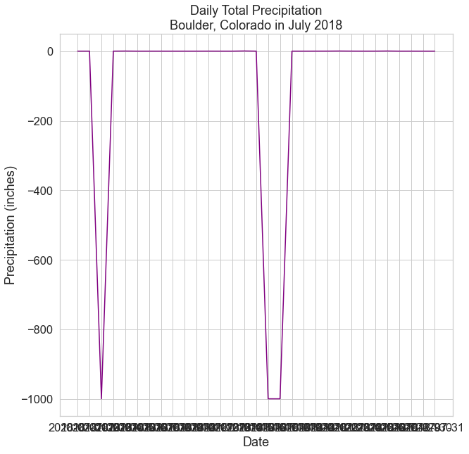
First, you will notice that there are many negative values in this dataset - these are actually “no data” values that you will handle in a later section on this page.
Now, look closely at the dates on the x-axis. When you plot a string field for the x-axis, Python gets stuck trying to plot the all of the date labels. Each value is read as a string, and it is difficult to try to fit all of those values on the x axis efficiently.
You can avoid this problem by converting the dates from strings to a datetime object during the import of data into a pandas dataframe. Once the dates are converted to a datetime object, you can more easily customize the dates on your plot, resulting in a more visually appealing plot.
Import Date Column into Pandas Dataframe As Datetime Object
To import the dates as a datetime object, you can use the parse_dates parameter of the pd.read_csv() function that allows you to indicate that a particular column should be converted to a datetime object:
parse_dates = ['date_column']
If you have a single column that contain dates in your data, you can also set dates as the index for the dataframe using the index_col parameter:
index_col = ['date_column']
You will use this index in later lessons to allow you to quickly summarize and aggregate your data by date.
Now you can recreate the dataframe using the parameter parse_datesto convert the dates from strings to datetime values and index_col to set the index of the dataframe to the datetime values.
# Import data using datetime and set index to datetime
boulder_july_2018 = pd.read_csv(file_path,
                                parse_dates=['date'],
                                index_col=['date'])

boulder_july_2018.head()
| max_temp | precip | |
|---|---|---|
| date | ||
| 2018-07-01 | 87 | 0.00 |
| 2018-07-02 | 92 | 0.00 |
| 2018-07-03 | 90 | -999.00 |
| 2018-07-04 | 87 | 0.00 |
| 2018-07-05 | 84 | 0.24 |
Notice that during the import, you converted the column date to the type datetime and you also set the index of the dataframe as that datetime object.
So rather than the index being the original RangeIndex of values from 0 to 31, the index is now a DatetimeIndex.
# View dataframe info
boulder_july_2018.info()
<class 'pandas.core.frame.DataFrame'>
DatetimeIndex: 31 entries, 2018-07-01 to 2018-07-31
Data columns (total 2 columns):
 #   Column    Non-Null Count  Dtype
---  ------    --------------  -----
 0   max_temp  31 non-null     int64
 1   precip    31 non-null     float64
dtypes: float64(1), int64(1)
memory usage: 744.0 bytes
Recall that after you set an index from a column in a dataframe, that original column is no longer listed as a column but rather is identified as the index of the dataframe.
# View column data types
boulder_july_2018.dtypes
max_temp      int64
precip      float64
dtype: object
Don’t worry - the data are still there! To check the values of an index of a dataframe, you can use the attribute index:
# View dataframe index
boulder_july_2018.index
DatetimeIndex(['2018-07-01', '2018-07-02', '2018-07-03', '2018-07-04',
               '2018-07-05', '2018-07-06', '2018-07-07', '2018-07-08',
               '2018-07-09', '2018-07-10', '2018-07-11', '2018-07-12',
               '2018-07-13', '2018-07-14', '2018-07-15', '2018-07-16',
               '2018-07-17', '2018-07-18', '2018-07-19', '2018-07-20',
               '2018-07-21', '2018-07-22', '2018-07-23', '2018-07-24',
               '2018-07-25', '2018-07-26', '2018-07-27', '2018-07-28',
               '2018-07-29', '2018-07-30', '2018-07-31'],
              dtype='datetime64[ns]', name='date', freq=None)
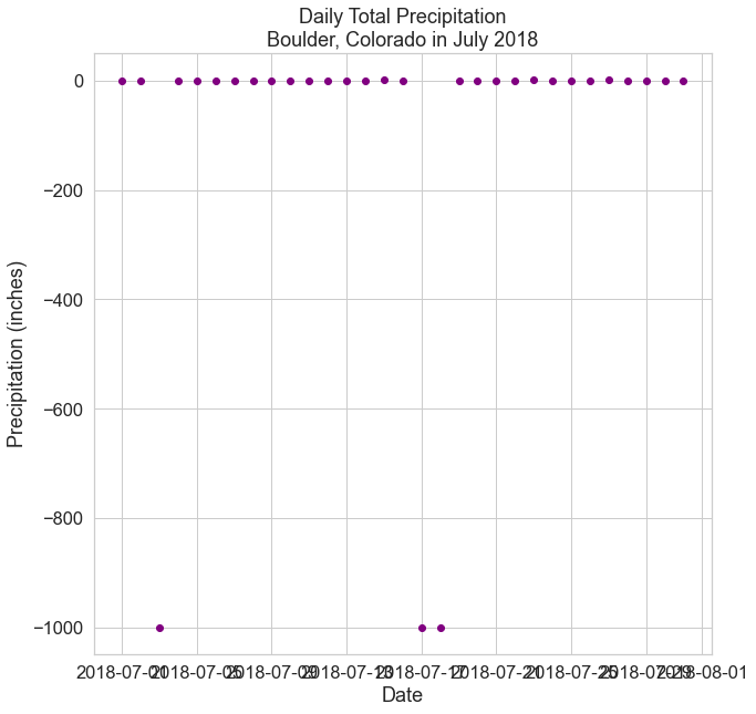
Plot Dates From Pandas Dataframe Using Datetime
In matplotlib, there are slight differences in how bar and scatter plots read in data versus how line plots read in data.
When plotting with ax.bar() and ax.scatter(), numpy is used to concatenate (a fancy word for combine) an array that has been created and passed in for the x-axis and/or y-axis data. However, numpy cannot concatenate the datetime object with other values.
Thus, if you try to pass a datetime column or index directly to ax.bar() or ax.scatter(), you will receive an error.
Use Index Values Attribute to Plot Datetime
To avoid this error, you can call the attribute .values on the datetime index using:
df.index.values
Notice that here you use df.index to access the datetime column because you have assigned your date column to be an index for the dataframe.
Also, notice that the spacing on the x-axis looks better and that your x-axis date labels are easier to read, as Python knows how to only show incremental values using datetime, rather than plotting each and every date value.
# Create figure and plot space
fig, ax = plt.subplots(figsize=(10, 10))

# Add x-axis and y-axis
ax.scatter(boulder_july_2018.index.values,
        boulder_july_2018['precip'],
        color='purple')

# Set title and labels for axes
ax.set(xlabel="Date",
       ylabel="Precipitation (inches)",
       title="Daily Total Precipitation\nBoulder, Colorado in July 2018")

plt.show()
# Create figure and plot space
fig, ax = plt.subplots(figsize=(10, 10))

# Add x-axis and y-axis
ax.bar(boulder_july_2018.index.values,
        boulder_july_2018['precip'],
        color='purple')

# Set title and labels for axes
ax.set(xlabel="Date",
       ylabel="Precipitation (inches)",
       title="Daily Total Precipitation\nBoulder, Colorado in July 2018")

# Rotate tick marks on x-axis
plt.setp(ax.get_xticklabels(), rotation=45)

plt.show()
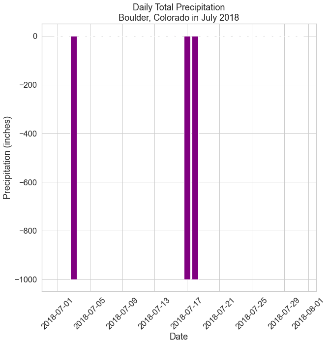
Note: you do not need to use .values when using an index that contains float values, rather than datetime objects, nor when creating a line graph using ax.plot().
However, for consistency of the code, the plot examples in this chapter will use index.values to create all plots using an index.
On later pages of this chapter, you will learn how to customize the date labels even more, such as displaying only month and day values or specifying the spacing for the time interval (i.e. frequency).
Work With No Data Values in Pandas Dataframe
As mentioned previously, you likely noticed that there are many negative values in this dataset, which are actually “no data” values.
Sometimes data are missing from a file due to errors in collection, inability to record a data point, or other reasons. For example, imagine a spreadsheet with cells that are blank. If the cells are blank, you don’t know for sure whether those data weren’t collected, or whether someone forgot to fill them in.
To account for data that are missing (not by mistake), you can put a value into those cells that represents “no data” to make it clear that these data are not usable for analysis or plotting.
Often, you’ll find a dataset that uses a specific value for “no data”. In many scientific disciplines, the value -999 is often used to indicate “no data” values.
In the example on this page, the data in july-2018-temperature-precip.csv contains “no data” values in the precip column using the value -999.
If you do not specify that the value -999 is the “no data” value, the values will be imported as real data, which will impact any statistics, calculations, and plots using the data.
For example, explore the data using describe() to see the impact of reading in those -999 values as true values.
# Both min and mean are affected by these negative, no data values
boulder_july_2018.describe()
| max_temp | precip | |
|---|---|---|
| count | 31.000000 | 31.000000 |
| mean | 88.129032 | -96.618065 |
| std | 6.626925 | 300.256388 |
| min | 75.000000 | -999.000000 |
| 25% | 84.000000 | 0.000000 |
| 50% | 88.000000 | 0.000000 |
| 75% | 94.000000 | 0.050000 |
| max | 97.000000 | 0.450000 |
The -999 values were imported as numeric values into the pandas dataframe when it was created, and thus, these values are included in the summary statistics.
To ensure “no data” values are properly ignored in your summary statistics, you can specify a “no data” value during the import, so that those values are not read as true numeric values using the parameter na_values as follows:
na_values = value
For example:
na_values = -999
This will tell pandas to treat all values of -999 as no data, and thus, not to include them in the analysis or on a plot.
Now that you know how to handle “no data” values, recreate the dataframe once more by including a value for the parameter na_values.
# Import data using datetime and no data value
boulder_july_2018 = pd.read_csv(file_path,
                                parse_dates=['date'],
                                index_col=['date'],
                                na_values=[-999])

boulder_july_2018.head()
| max_temp | precip | |
|---|---|---|
| date | ||
| 2018-07-01 | 87 | 0.00 |
| 2018-07-02 | 92 | 0.00 |
| 2018-07-03 | 90 | NaN |
| 2018-07-04 | 87 | 0.00 |
| 2018-07-05 | 84 | 0.24 |
Notice that the -999 value for precip on July 3rd has been replaced with NaN to indicate a “no data” value.
Now have a look at the summary statistics.
# Both min and mean now accurately reflect the true data
boulder_july_2018.describe()
| max_temp | precip | |
|---|---|---|
| count | 31.000000 | 28.000000 |
| mean | 88.129032 | 0.065714 |
| std | 6.626925 | 0.120936 |
| min | 75.000000 | 0.000000 |
| 25% | 84.000000 | 0.000000 |
| 50% | 88.000000 | 0.000000 |
| 75% | 94.000000 | 0.055000 |
| max | 97.000000 | 0.450000 |
Finally, plot the data one last time to see that the negative values -999 are no longer on the plot.
# Create figure and plot space
fig, ax = plt.subplots(figsize=(10, 10))

# Add x-axis and y-axis
ax.scatter(boulder_july_2018.index.values,
        boulder_july_2018['precip'],
        color='purple')

# Set title and labels for axes
ax.set(xlabel="Date",
       ylabel="Precipitation (inches)",
       title="Daily Total Precipitation\nBoulder, Colorado in July 2018")

plt.show()
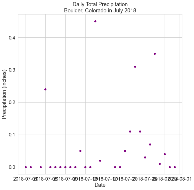
By using the na_values parameter, you told Python to ignore those “no data” values (which are now labeled as NaN) when it performs calculations on the data and when it plots the data.
Note: if there are multiple types of missing values in your dataset, you can add multiple values in the na_values parameter as follows:
na_values=['NA', ' ', -999])
which would specify that the “no data” values are “NA” as a string, an empty space as a string, or the numeric value -999.
You now know how to import dates into pandas dataframes using the datetime object in Python and how to deal with no data values.
On the next pages of this chapter, you will learn more about working with datetime in Python to temporally subset and resample data as well as customize your plots even more.
Share on
Twitter Facebook Google+ LinkedIn
Leave a Comment