Lesson 4. Crop Spatial Raster Data With a Shapefile in Python
Learning Objectives
- Crop a raster dataset in Python using a vector extent object derived from a shapefile.
- Open a shapefile in Python.
In previous lessons, you reclassified a raster in Python; however, the edges of your raster dataset were uneven.
In this lesson, you will learn how to crop a raster - to create a new raster object / file that you can share with colleagues and / or open in other tools such as a Desktop GIS tool like QGIS.
About Spatial Crop
Cropping (sometimes also referred to as clipping), is when you subset or make a dataset smaller, by removing all data outside of the crop area or spatial extent. In this case you have a large raster - but let’s pretend that you only need to work with a smaller subset of the raster.
You can use the crop_image function to remove all of the data outside of your study area.
This is useful as it:
- Makes the data smaller and
- Makes processing and plotting faster
In general when you can, it’s often a good idea to crop your raster data!
To begin let’s load the libraries that you will need in this lesson.
Load Libraries
import os
import matplotlib.pyplot as plt
import seaborn as sns
import numpy as np
from shapely.geometry import mapping
import rioxarray as rxr
import xarray as xr
import geopandas as gpd

import earthpy as et
import earthpy.plot as ep

# Prettier plotting with seaborn
sns.set(font_scale=1.5)

# Get data and set working directory
et.data.get_data("colorado-flood")
os.chdir(os.path.join(et.io.HOME,
                      'earth-analytics',
                      'data'))
Downloading from https://ndownloader.figshare.com/files/16371473
Extracted output to /root/earth-analytics/data/colorado-flood/.
Open Raster and Vector Layers
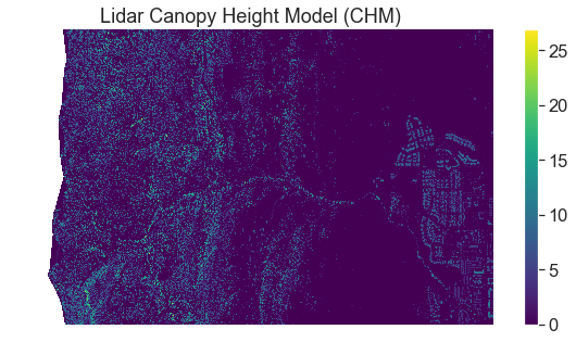
In the previous lessons, you worked with a raster layer that looked like the one below. Notice that the data have an uneven edge on the left hand side. Let’s pretend this edge is outside of your study area and you’d like to remove it or clip it off using your study area extent. You can do this using the crop_image() function in earthpy.spatial.
lidar_chm_path = os.path.join("colorado-flood",
                              "spatial"
                              "boulder-leehill-rd",
                              "outputs",
                              "lidar_chm.tif")

lidar_chm_im = rxr.open_rasterio("colorado-flood/spatial/boulder-leehill-rd/outputs/lidar_chm.tif",
                                 masked=True).squeeze()

f, ax = plt.subplots(figsize=(10, 5))
lidar_chm_im.plot.imshow()
ax.set(title="Lidar Canopy Height Model (CHM)")

ax.set_axis_off()
plt.show()
Open Vector Layer
To begin your clip, open up a vector layer that contains the crop extent that you want
to use to crop your data. To open a shapefile you use the gpd.read_file() function
from geopandas. You will learn more about vector data in Python in a few weeks.
aoi = os.path.join("colorado-flood",
                   "spatial",
                   "boulder-leehill-rd",
                   "clip-extent.shp")

# Open crop extent (your study area extent boundary)
crop_extent = gpd.read_file(aoi)
Next, view the coordinate reference system (CRS) of both of your datasets. Remember that in order to perform any analysis with these two datasets together, they will need to be in the same CRS.
print('crop extent crs: ', crop_extent.crs)
print('lidar crs: ', lidar_chm_im.rio.crs)
crop extent crs:  epsg:32613
lidar crs:  EPSG:32613
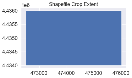
# Plot the crop boundary layer
# Note this is just an example so you can see what it looks like
# You don't need to plot this layer in your homework!
fig, ax = plt.subplots(figsize=(6, 6))

crop_extent.plot(ax=ax)

ax.set_title("Shapefile Crop Extent",
             fontsize=16)
plt.show()
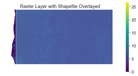
Now that you have imported the shapefile. You can use the crop_image function from earthpy.spatial to crop the raster data using the vector shapefile.
f, ax = plt.subplots(figsize=(10, 5))
lidar_chm_im.plot.imshow(ax=ax)

crop_extent.plot(ax=ax,
                 alpha=.8)
ax.set(title="Raster Layer with Shapefile Overlayed")

ax.set_axis_off()
plt.show()
Clip Raster Data Using RioXarray .clip
If you want to crop the data you can use the rio.clip function. When you clip
the data, you can then export it and share it with colleagues. Or use it in
another analysis.
To perform the clip you:
- Open the raster dataset that you wish to crop using xarray or rioxarray.
- Open your shapefile as a geopandas object.
- Crop the data using the
.clip()function.
.clip has several parameters that you can consider including
drop = True: The default. setting it will drop all pixels outside of the clip extentinvert = False: The default. If set to true it will clip all data INSIDE of the clip extentcrs: if your shapefile is in a different CRS than the raster data, pass the CRS to ensure the data are clipped correctly.
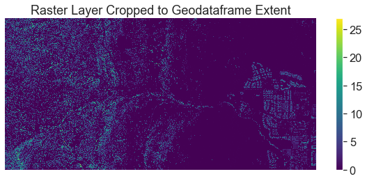
Below you clip the data to the extent of the AOI geodataframe imported above. The data are then plotted.
lidar_clipped = lidar_chm_im.rio.clip(crop_extent.geometry.apply(mapping),
                                      # This is needed if your GDF is in a diff CRS than the raster data
                                      crop_extent.crs)

f, ax = plt.subplots(figsize=(10, 4))
lidar_clipped.plot(ax=ax)
ax.set(title="Raster Layer Cropped to Geodataframe Extent")
ax.set_axis_off()
plt.show()
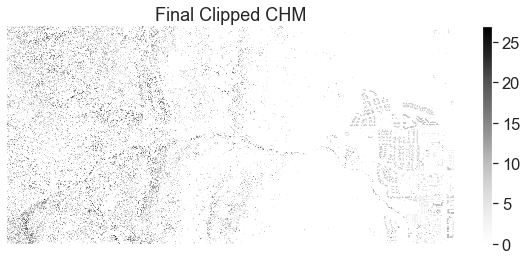
OPTIONAL – Export Newly Cropped Raster
Once you have cropped your data, you may want to export it to a new geotiff file, just like you did in previous lessons.
You can so this using rioxarray too!
path_to_tif_file = os.path.join("colorado-flood",
                                "spatial",
                                "outputs",
                                "lidar_chm_cropped.tif")

# Write the data to a new geotiff file
lidar_clipped.rio.to_raster(path_to_tif_file)
# Open the data you wrote out above
clipped_chm = rxr.open_rasterio(path_to_tif_file)

# Customize your plot as you wish!
f, ax = plt.subplots(figsize=(10, 4))
clipped_chm.plot(ax=ax,
                 cmap='Greys')
ax.set(title="Final Clipped CHM")
ax.set_axis_off()
plt.show()
Optional Challenge: Crop Change Over Time Layers
In the previous lesson, you created 2 plots:
- A classified raster map that shows positive and negative change in the canopy height model before and after the flood. To do this you will need to calculate the difference between two canopy height models.
- A classified raster map that shows positive and negative change in terrain extracted from the pre and post flood Digital Terrain Models before and after the flood.
Create the same two plots except this time CROP each of the rasters that you plotted
using the shapefile: data/week-03/boulder-leehill-rd/crop_extent.shp
For each plot, be sure to:
- Add a legend that clearly shows what each color in your classified raster represents.
- Use proper colors.
- Add a title to your plot.
You will include these plots in your final report due next week.
Share on
Twitter Facebook Google+ LinkedIn
Leave a Comment