Lesson 2. Open and Crop Landsat Remote Sensing Data in Open Source Python
Learning Objectives
After completing this lesson, you will be able to:
- Create a list of subsets of landsat
.tiffiles usingglobandos.path.join - Crop xarray objects.
- Stack a list of landsat
.tiffiles into a xarray object. - Create a workflow that opens, stacks and cleans landsat data efficiently.
Open Landsat .tif Files in Python
It’s time to get start processing your data. To begin, load your libraries and set up your working directory.
import os
from glob import glob

import matplotlib.pyplot as plt
import geopandas as gpd
import rasterio as rio
import xarray as xr
import rioxarray as rxr
import numpy as np
import earthpy as et
import earthpy.spatial as es
import earthpy.plot as ep
from shapely.geometry import mapping


# Download data and set working directory
data = et.data.get_data('cold-springs-fire')
os.chdir(os.path.join(et.io.HOME,
                      'earth-analytics',
                      'data'))
You will be working in the landsat-collect directory. Notice that the data in that directory are stored by individual band. Each file is a single geotiff (.tif) rather than one tif with all the bands which is what you worked with in the previous lesson with NAIP data.
Why Are Landsat Bands Stored As Individual Files?
Originally Landsat was stored in a file format called HDF - hierarchical
data format. However that format, while extremely efficient, is a bit more
challenging to work with. In recent years, USGS has started to make each band
of a landsat scene available as a .tif file. This makes it a bit easier to use
across many different programs and platforms.
The good news is that you already know how to work with .tif files in Python. You just need to learn how to batch process a series of .tif files to work with Landsat 8 Collections.
Generate a List of Files in Python
To begin, explore the Landsat files in your cs-test-landsat directory. Start with the data:
data/cs-test-landsat/
Landsat scenes are large. In order to make processing your data more efficient, you can subset the data to just the parts that you need. This may include:
- only opening bands that you need for your final analysis and
- cropping the data if your study area is small than or not fully covered by the landsat scene extent.
For the purpose of this lesson, let’s pretend that you wish to perform an NDVI analysis of your Landsat data. You also may wish to plot Color infrared images and an RGB image. To perform this you will want to grab the following bands:
- Red, green, blue and near infrared
from your data. This should be bands 2-5 following the landsat documentation.
Below are all of the bands in your landsat data:
'LC08_L1TP_034032_20160621_20170221_01_T1_sr_band7.tif',
'LC08_L1TP_034032_20160621_20170221_01_T1.xml',
'LC08_L1TP_034032_20160621_20170221_01_T1_sr_band5.tif',
'LC08_L1TP_034032_20160621_20170221_01_T1_sr_band1.tif',
'LC08_L1TP_034032_20160621_20170221_01_T1_sr_aerosol.tif',
'LC08_L1TP_034032_20160621_20170221_01_T1_sr_band3.tif',
'LC08_L1TP_034032_20160621_20170221_01_T1_ANG.txt',
'LC08_L1TP_034032_20160621_20170221_01_T1_sr_band2.tif',
'crop',
'LC08_L1TP_034032_20160621_20170221_01_T1_sr_band4.tif',
'LC08_L1TP_034032_20160621_20170221_01_T1_sr_band6.tif',
'LC08_L1TP_034032_20160621_20170221_01_T1_pixel_qa.tif',
'LC08_L1TP_034032_20160621_20170221_01_T1_radsat_qa.tif',
'LC08_L1TP_034032_20160621_20170221_01_T1_MTL.txt'
Notice that there are some layers that are quality assurance layers. Others have the word band in them. The layers with band in them are the reflectance data that you need to work with.
To work with these files, you will do the following:
- You will generate a list of only the files in the directory that contain the word band in the name and that only represent the bands that you need for your analysis.
- Crop the data to the extent of the study area.
- OPTIONAL: stack all of the layers into one rioxarray object: Note that you may or may not wish to stack the data. If your main goal is to calculate NDVI, or some other vegetation index, then stacking may not be necessary. If you wish to create color plots of your data in RGB or CIR format, or to perform other analytics on the stacked data then it may make sense to stack the data.
You will use the glob() function and library to do this in Python.
Begin exploring your data by grabbing all of the files in the directory using /*.
landsat_post_fire_path = os.path.join("cold-springs-fire",
                                      "landsat_collect",
                                      "LC080340322016072301T1-SC20180214145802",
                                      "crop")

glob(os.path.join(landsat_post_fire_path, "*"))
['cold-springs-fire/landsat_collect/LC080340322016072301T1-SC20180214145802/crop/LC08_L1TP_034032_20160723_20180131_01_T1_pixel_qa_crop.tif',
 'cold-springs-fire/landsat_collect/LC080340322016072301T1-SC20180214145802/crop/LC08_L1TP_034032_20160723_20180131_01_T1_radsat_qa_crop.tif',
 'cold-springs-fire/landsat_collect/LC080340322016072301T1-SC20180214145802/crop/LC08_L1TP_034032_20160723_20180131_01_T1_sr_aerosol_crop.tif',
 'cold-springs-fire/landsat_collect/LC080340322016072301T1-SC20180214145802/crop/LC08_L1TP_034032_20160723_20180131_01_T1_sr_band1_crop.tif',
 'cold-springs-fire/landsat_collect/LC080340322016072301T1-SC20180214145802/crop/LC08_L1TP_034032_20160723_20180131_01_T1_sr_band2_crop.tif',
 'cold-springs-fire/landsat_collect/LC080340322016072301T1-SC20180214145802/crop/LC08_L1TP_034032_20160723_20180131_01_T1_sr_band3_crop.tif',
 'cold-springs-fire/landsat_collect/LC080340322016072301T1-SC20180214145802/crop/LC08_L1TP_034032_20160723_20180131_01_T1_sr_band4_crop.tif',
 'cold-springs-fire/landsat_collect/LC080340322016072301T1-SC20180214145802/crop/LC08_L1TP_034032_20160723_20180131_01_T1_sr_band5_crop.tif',
 'cold-springs-fire/landsat_collect/LC080340322016072301T1-SC20180214145802/crop/LC08_L1TP_034032_20160723_20180131_01_T1_sr_band6_crop.tif',
 'cold-springs-fire/landsat_collect/LC080340322016072301T1-SC20180214145802/crop/LC08_L1TP_034032_20160723_20180131_01_T1_sr_band7_crop.tif']
Grab Subsets of File Names Using File Names and Other Criteria
Above you generated a list of all files in the directory. However, you may want to subset that list to only include:
.tiffiles.tiffiles that contain the word “band” in them
Note that it is important that the file ends with .tif. So we use an asterisk at the end of the path to tell Python to only grab files that end with .tif.
path/*.tif will grab all files in the crop directory that end with the .tif extension.
glob(os.path.join(landsat_post_fire_path, "*.tif"))
['cold-springs-fire/landsat_collect/LC080340322016072301T1-SC20180214145802/crop/LC08_L1TP_034032_20160723_20180131_01_T1_pixel_qa_crop.tif',
 'cold-springs-fire/landsat_collect/LC080340322016072301T1-SC20180214145802/crop/LC08_L1TP_034032_20160723_20180131_01_T1_radsat_qa_crop.tif',
 'cold-springs-fire/landsat_collect/LC080340322016072301T1-SC20180214145802/crop/LC08_L1TP_034032_20160723_20180131_01_T1_sr_aerosol_crop.tif',
 'cold-springs-fire/landsat_collect/LC080340322016072301T1-SC20180214145802/crop/LC08_L1TP_034032_20160723_20180131_01_T1_sr_band1_crop.tif',
 'cold-springs-fire/landsat_collect/LC080340322016072301T1-SC20180214145802/crop/LC08_L1TP_034032_20160723_20180131_01_T1_sr_band2_crop.tif',
 'cold-springs-fire/landsat_collect/LC080340322016072301T1-SC20180214145802/crop/LC08_L1TP_034032_20160723_20180131_01_T1_sr_band3_crop.tif',
 'cold-springs-fire/landsat_collect/LC080340322016072301T1-SC20180214145802/crop/LC08_L1TP_034032_20160723_20180131_01_T1_sr_band4_crop.tif',
 'cold-springs-fire/landsat_collect/LC080340322016072301T1-SC20180214145802/crop/LC08_L1TP_034032_20160723_20180131_01_T1_sr_band5_crop.tif',
 'cold-springs-fire/landsat_collect/LC080340322016072301T1-SC20180214145802/crop/LC08_L1TP_034032_20160723_20180131_01_T1_sr_band6_crop.tif',
 'cold-springs-fire/landsat_collect/LC080340322016072301T1-SC20180214145802/crop/LC08_L1TP_034032_20160723_20180131_01_T1_sr_band7_crop.tif']
To only grab files containing the word band AND that end with .tif we use *band*.tif.
This tells python to look for the word band anywhere before the .tif extension AND anywhere within the file name. You can use number ranges to JUST get the bands you need. For this exercise, we will use all of the bands. But if you were just working with RGB images, you could filter this further by specifying *band[2-5]*.tif.
# Only grab bands 2 through 5
all_landsat_post_bands = glob(os.path.join(landsat_post_fire_path,
                                           "*band[2-5]*.tif"))
all_landsat_post_bands
['cold-springs-fire/landsat_collect/LC080340322016072301T1-SC20180214145802/crop/LC08_L1TP_034032_20160723_20180131_01_T1_sr_band2_crop.tif',
 'cold-springs-fire/landsat_collect/LC080340322016072301T1-SC20180214145802/crop/LC08_L1TP_034032_20160723_20180131_01_T1_sr_band3_crop.tif',
 'cold-springs-fire/landsat_collect/LC080340322016072301T1-SC20180214145802/crop/LC08_L1TP_034032_20160723_20180131_01_T1_sr_band4_crop.tif',
 'cold-springs-fire/landsat_collect/LC080340322016072301T1-SC20180214145802/crop/LC08_L1TP_034032_20160723_20180131_01_T1_sr_band5_crop.tif']
Be sure that your bands are in numerical band order starting at
1 and ending at 7! If the data are not in order, you can use the .sort()
list method to sort your list alphabetically. The data in this lesson
are sorted properly; however, we have noticed that this sort doesn’t
happen by default on some machines. The code below will sort your list
of band paths.
all_landsat_post_bands.sort()
all_landsat_post_bands
['cold-springs-fire/landsat_collect/LC080340322016072301T1-SC20180214145802/crop/LC08_L1TP_034032_20160723_20180131_01_T1_sr_band2_crop.tif',
 'cold-springs-fire/landsat_collect/LC080340322016072301T1-SC20180214145802/crop/LC08_L1TP_034032_20160723_20180131_01_T1_sr_band3_crop.tif',
 'cold-springs-fire/landsat_collect/LC080340322016072301T1-SC20180214145802/crop/LC08_L1TP_034032_20160723_20180131_01_T1_sr_band4_crop.tif',
 'cold-springs-fire/landsat_collect/LC080340322016072301T1-SC20180214145802/crop/LC08_L1TP_034032_20160723_20180131_01_T1_sr_band5_crop.tif']
In the previous lesson, you created a small function that opened up a single landsat band. You will expand this function to open, crop and clean your data in this lesson.
def open_clean_band(band_path):
    """A function that opens a Landsat band as an (rio)xarray object

    Parameters
    ----------
    band_path : list
        A list of paths to the tif files that you wish to combine.

    Returns
    -------
    An single xarray object with the Landsat band data.

    """

    return rxr.open_rasterio(band_path, masked=True).squeeze()
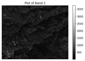
landsat_post_xr = open_clean_band(all_landsat_post_bands[0])

# Plot the data
f, ax = plt.subplots()
landsat_post_xr.plot.imshow(cmap="Greys_r",
                            ax=ax)
ax.set_title("Plot of Band 2")
ax.set_axis_off()
plt.show()
Crop a Landsat Band Using Rioxarray rio.clip()
Above you opened up and plotted a single band. Often, you want to crop
your data to the spatial extent of your study area. Crop, removes data that you
don’t need in your analysis (that that is outside of your area of interest).
You could chose to open and crop each file individually using the
rxr.open_rasterio() function alongside
the rioxarray opened_xarray.rio.clip() function as shown below.
In order to crop a band, you need to have a
- GeoPandas or shapely object that represents the extent of the area you want to study in the Landsat image (your crop extent).
- The crop extent shapefile and the Landsat data need to be in the same Coordinate Reference System, or CRS.
To clip an xarray DataFrame to a GeoPandas extent, you need to create the clipped dataframe with the following syntax.
clipped_xarray = xarray_name.rio.clip(geopandas_object_name.geometry)
HINT: You can retrieve the CRS of your Landsat data using es.crs_check(landsat_band_path).
Below you crop your stacked data using a shapefile.
# Open up boundary extent using GeoPandas
fire_boundary_path = os.path.join("cold-springs-fire",
                                  "vector_layers",
                                  "fire-boundary-geomac",
                                  "co_cold_springs_20160711_2200_dd83.shp")

fire_boundary = gpd.read_file(fire_boundary_path)
# Get the CRS of your data
landsat_crs = es.crs_check(all_landsat_post_bands[0])

print("Landsat crs is:", landsat_crs)
print("Fire boundary crs", fire_boundary.crs)
Landsat crs is: EPSG:32613
Fire boundary crs epsg:4269
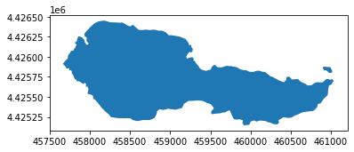
# Reproject data to CRS of raster data
fire_boundary_utmz13 = fire_boundary.to_crs(landsat_crs)
fire_boundary_utmz13.plot()
plt.show()
Once the crs has been checked you can clip the data. The ideal scenario
here is that you clip the data while opening it. Below you use
from_disk = True which tells rioxarray to only open the data within the
clip extent. This will speed up your workflow a bit.
landsat_post_xr_clip = rxr.open_rasterio(all_landsat_post_bands[0]).rio.clip(
    fire_boundary_utmz13.geometry,
    from_disk=True).squeeze()

# Notice the x and y data dimensions of your data have changed
landsat_post_xr_clip
<xarray.DataArray (y: 44, x: 113)>
array([[-32768, -32768, -32768, ..., -32768, -32768, -32768],
       [-32768, -32768, -32768, ..., -32768, -32768, -32768],
       [-32768, -32768, -32768, ..., -32768, -32768, -32768],
       ...,
       [-32768, -32768, -32768, ..., -32768, -32768, -32768],
       [-32768, -32768, -32768, ..., -32768, -32768, -32768],
       [-32768, -32768, -32768, ..., -32768, -32768, -32768]], dtype=int16)
Coordinates:
  * x            (x) float64 4.577e+05 4.577e+05 4.577e+05 ... 4.61e+05 4.61e+05
  * y            (y) float64 4.426e+06 4.426e+06 ... 4.425e+06 4.425e+06
    band         int64 1
    spatial_ref  int64 0
Attributes:
    STATISTICS_MAXIMUM:  3743
    STATISTICS_MEAN:     337.61331587892
    STATISTICS_MINIMUM:  17
    STATISTICS_STDDEV:   139.84903539903
    scale_factor:        1.0
    add_offset:          0.0
_FillValue: -32768- y: 44
- x: 113
- -32768 -32768 -32768 -32768 -32768 ... -32768 -32768 -32768 -32768
array([[-32768, -32768, -32768, ..., -32768, -32768, -32768], [-32768, -32768, -32768, ..., -32768, -32768, -32768], [-32768, -32768, -32768, ..., -32768, -32768, -32768], ..., [-32768, -32768, -32768, ..., -32768, -32768, -32768], [-32768, -32768, -32768, ..., -32768, -32768, -32768], [-32768, -32768, -32768, ..., -32768, -32768, -32768]], dtype=int16) - x(x)float644.577e+05 4.577e+05 ... 4.61e+05
- axis :
- X
- long_name :
- x coordinate of projection
- standard_name :
- projection_x_coordinate
- units :
- metre
array([457680., 457710., 457740., 457770., 457800., 457830., 457860., 457890., 457920., 457950., 457980., 458010., 458040., 458070., 458100., 458130., 458160., 458190., 458220., 458250., 458280., 458310., 458340., 458370., 458400., 458430., 458460., 458490., 458520., 458550., 458580., 458610., 458640., 458670., 458700., 458730., 458760., 458790., 458820., 458850., 458880., 458910., 458940., 458970., 459000., 459030., 459060., 459090., 459120., 459150., 459180., 459210., 459240., 459270., 459300., 459330., 459360., 459390., 459420., 459450., 459480., 459510., 459540., 459570., 459600., 459630., 459660., 459690., 459720., 459750., 459780., 459810., 459840., 459870., 459900., 459930., 459960., 459990., 460020., 460050., 460080., 460110., 460140., 460170., 460200., 460230., 460260., 460290., 460320., 460350., 460380., 460410., 460440., 460470., 460500., 460530., 460560., 460590., 460620., 460650., 460680., 460710., 460740., 460770., 460800., 460830., 460860., 460890., 460920., 460950., 460980., 461010., 461040.]) - y(y)float644.426e+06 4.426e+06 ... 4.425e+06
- axis :
- Y
- long_name :
- y coordinate of projection
- standard_name :
- projection_y_coordinate
- units :
- metre
array([4426440., 4426410., 4426380., 4426350., 4426320., 4426290., 4426260., 4426230., 4426200., 4426170., 4426140., 4426110., 4426080., 4426050., 4426020., 4425990., 4425960., 4425930., 4425900., 4425870., 4425840., 4425810., 4425780., 4425750., 4425720., 4425690., 4425660., 4425630., 4425600., 4425570., 4425540., 4425510., 4425480., 4425450., 4425420., 4425390., 4425360., 4425330., 4425300., 4425270., 4425240., 4425210., 4425180., 4425150.]) - band()int641
array(1)
- spatial_ref()int640
- crs_wkt :
- PROJCS["WGS 84 / UTM zone 13N",GEOGCS["WGS 84",DATUM["WGS_1984",SPHEROID["WGS 84",6378137,298.257223563,AUTHORITY["EPSG","7030"]],AUTHORITY["EPSG","6326"]],PRIMEM["Greenwich",0,AUTHORITY["EPSG","8901"]],UNIT["degree",0.0174532925199433,AUTHORITY["EPSG","9122"]],AUTHORITY["EPSG","4326"]],PROJECTION["Transverse_Mercator"],PARAMETER["latitude_of_origin",0],PARAMETER["central_meridian",-105],PARAMETER["scale_factor",0.9996],PARAMETER["false_easting",500000],PARAMETER["false_northing",0],UNIT["metre",1,AUTHORITY["EPSG","9001"]],AXIS["Easting",EAST],AXIS["Northing",NORTH],AUTHORITY["EPSG","32613"]]
- semi_major_axis :
- 6378137.0
- semi_minor_axis :
- 6356752.314245179
- inverse_flattening :
- 298.257223563
- reference_ellipsoid_name :
- WGS 84
- longitude_of_prime_meridian :
- 0.0
- prime_meridian_name :
- Greenwich
- geographic_crs_name :
- WGS 84
- horizontal_datum_name :
- World Geodetic System 1984
- projected_crs_name :
- WGS 84 / UTM zone 13N
- grid_mapping_name :
- transverse_mercator
- latitude_of_projection_origin :
- 0.0
- longitude_of_central_meridian :
- -105.0
- false_easting :
- 500000.0
- false_northing :
- 0.0
- scale_factor_at_central_meridian :
- 0.9996
- spatial_ref :
- PROJCS["WGS 84 / UTM zone 13N",GEOGCS["WGS 84",DATUM["WGS_1984",SPHEROID["WGS 84",6378137,298.257223563,AUTHORITY["EPSG","7030"]],AUTHORITY["EPSG","6326"]],PRIMEM["Greenwich",0,AUTHORITY["EPSG","8901"]],UNIT["degree",0.0174532925199433,AUTHORITY["EPSG","9122"]],AUTHORITY["EPSG","4326"]],PROJECTION["Transverse_Mercator"],PARAMETER["latitude_of_origin",0],PARAMETER["central_meridian",-105],PARAMETER["scale_factor",0.9996],PARAMETER["false_easting",500000],PARAMETER["false_northing",0],UNIT["metre",1,AUTHORITY["EPSG","9001"]],AXIS["Easting",EAST],AXIS["Northing",NORTH],AUTHORITY["EPSG","32613"]]
- GeoTransform :
- 457665.0 30.0 0.0 4426455.0 0.0 -30.0
array(0)
- STATISTICS_MAXIMUM :
- 3743
- STATISTICS_MEAN :
- 337.61331587892
- STATISTICS_MINIMUM :
- 17
- STATISTICS_STDDEV :
- 139.84903539903
- scale_factor :
- 1.0
- add_offset :
- 0.0
- _FillValue :
- -32768
Now that your data are open, you can plot it.
# Plot the data
f, ax = plt.subplots(figsize=(10, 6))
landsat_post_xr_clip.plot.imshow(cmap="Greys_r",
                                 ax=ax)
ax.set_axis_off()
ax.set_title("Band 1 - Clipped To Your Study Area")
plt.show()
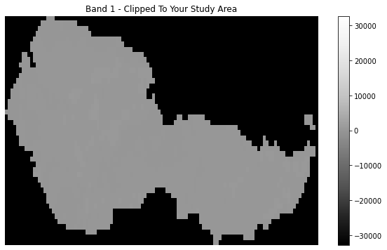
The above plot has a large amount of “black” fill around the outside representing fill values. When you clipped the data to the geometry, rioxarray filled all of the pixels outside of the geometry extent with a large negative number -32768.
For plotting you may wish to clean this up by masking out values.
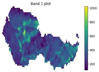
# Clean the data
valid_range = (0, 10000)
# Only run this step if a valid range tuple is provided
if valid_range:
    mask = ((landsat_post_xr_clip < valid_range[0]) | (
        landsat_post_xr_clip > valid_range[1]))
    landsat_post_xr_clip = landsat_post_xr_clip.where(
        ~xr.where(mask, True, False))
f, ax = plt.subplots()
landsat_post_xr_clip.plot(ax=ax)
ax.set_title("Band 1 plot")
ax.set_axis_off()
plt.show()

A Function to Crop and Clean Landsat Data
It would be nice to combine all of the steps above into a single
workflow that clips and cleans your landsat data. You can take the
function that you started in the previous lesson and expand it to
do all of this for you.
def open_clean_band(band_path, clip_extent, valid_range=None):
    """A function that opens a Landsat band as an (rio)xarray object

    Parameters
    ----------
    band_path : list
        A list of paths to the tif files that you wish to combine.

    clip_extent : geopandas geodataframe
        A geodataframe containing the clip extent of interest. NOTE: this will
        fail if the clip extent is in a different CRS than the raster data.

    valid_range : tuple (optional)
        The min and max valid range for the data. All pixels with values outside
        of this range will be masked.

    Returns
    -------
    An single xarray object with the Landsat band data.

    """

    try:
        clip_bound = clip_extent.geometry
    except Exception as err:
        print("Oops, I need a geodataframe object for this to work.")
        print(err)

    cleaned_band = rxr.open_rasterio(band_path,
                                     masked=True).rio.clip(clip_bound,
                                                           from_disk=True).squeeze()

    # Only mask the data if a valid range tuple is provided
    if valid_range:
        mask = ((landsat_post_xr_clip < valid_range[0]) | (
            landsat_post_xr_clip > valid_range[1]))
        cleaned_band = landsat_post_xr_clip.where(
            ~xr.where(mask, True, False))

    return cleaned_band
cleaned_band = open_clean_band(all_landsat_post_bands[0], fire_boundary_utmz13)

f, ax = plt.subplots()
cleaned_band.plot(ax=ax)
ax.set_title("Band 1 plot")
ax.set_axis_off()
plt.show()
Create Your Final, Automated Workflow
Great - you now have a workflow that opens, clips and cleans a single band.
However, remember that your original goal is to open, clip and clean several
Landsat bands with the goal of calculating NDVI and producing some RGB and
ColorInfrared (CIR) plots.
Below you build out the entire workflow using a loop. The vector data step is
reproduced here
# Open up boundary extent using GeoPandas
fire_boundary_path = os.path.join("cold-springs-fire",
                                  "vector_layers",
                                  "fire-boundary-geomac",
                                  "co_cold_springs_20160711_2200_dd83.shp")

fire_boundary = gpd.read_file(fire_boundary_path)
# Get a list of required bands - bands 2 through 5
all_landsat_post_bands = glob(os.path.join(landsat_post_fire_path,
                                           "*band[2-5]*.tif"))
all_landsat_post_bands.sort()
all_landsat_post_bands
['cold-springs-fire/landsat_collect/LC080340322016072301T1-SC20180214145802/crop/LC08_L1TP_034032_20160723_20180131_01_T1_sr_band2_crop.tif',
 'cold-springs-fire/landsat_collect/LC080340322016072301T1-SC20180214145802/crop/LC08_L1TP_034032_20160723_20180131_01_T1_sr_band3_crop.tif',
 'cold-springs-fire/landsat_collect/LC080340322016072301T1-SC20180214145802/crop/LC08_L1TP_034032_20160723_20180131_01_T1_sr_band4_crop.tif',
 'cold-springs-fire/landsat_collect/LC080340322016072301T1-SC20180214145802/crop/LC08_L1TP_034032_20160723_20180131_01_T1_sr_band5_crop.tif']
# Reproject your vector layer
landsat_crs = es.crs_check(all_landsat_post_bands[0])

# Reproject fire boundary for clipping
fire_boundary_utmz13 = fire_boundary.to_crs(landsat_crs)
Loop through each band path, open the data and add it to a list.
post_all_bands = []
for i, aband in enumerate(all_landsat_post_bands):
    cleaned = open_clean_band(aband, fire_boundary_utmz13)
    # This line below is only needed if you wish to stack and plot your data
    cleaned["band"] = i+1
    post_all_bands.append(cleaned)
Stack Your Final Cleaned Data
If you wish, you can stack all of the bands in your workflow by using the
xr.concat function. Stacking the data will store all bands in one single
xarray object. This step is optional and may be needed for some workflows
but not for others.
# OPTIONAL - Stack the data
post_fire_stack = xr.concat(post_all_bands, dim="band")
post_fire_stack
<xarray.DataArray (band: 4, y: 44, x: 113)>
array([[[nan, nan, nan, ..., nan, nan, nan],
        [nan, nan, nan, ..., nan, nan, nan],
        [nan, nan, nan, ..., nan, nan, nan],
        ...,
        [nan, nan, nan, ..., nan, nan, nan],
        [nan, nan, nan, ..., nan, nan, nan],
        [nan, nan, nan, ..., nan, nan, nan]],

       [[nan, nan, nan, ..., nan, nan, nan],
        [nan, nan, nan, ..., nan, nan, nan],
        [nan, nan, nan, ..., nan, nan, nan],
        ...,
        [nan, nan, nan, ..., nan, nan, nan],
        [nan, nan, nan, ..., nan, nan, nan],
        [nan, nan, nan, ..., nan, nan, nan]],

       [[nan, nan, nan, ..., nan, nan, nan],
        [nan, nan, nan, ..., nan, nan, nan],
        [nan, nan, nan, ..., nan, nan, nan],
        ...,
        [nan, nan, nan, ..., nan, nan, nan],
        [nan, nan, nan, ..., nan, nan, nan],
        [nan, nan, nan, ..., nan, nan, nan]],

       [[nan, nan, nan, ..., nan, nan, nan],
        [nan, nan, nan, ..., nan, nan, nan],
        [nan, nan, nan, ..., nan, nan, nan],
        ...,
        [nan, nan, nan, ..., nan, nan, nan],
        [nan, nan, nan, ..., nan, nan, nan],
        [nan, nan, nan, ..., nan, nan, nan]]])
Coordinates:
  * x            (x) float64 4.577e+05 4.577e+05 4.577e+05 ... 4.61e+05 4.61e+05
  * y            (y) float64 4.426e+06 4.426e+06 ... 4.425e+06 4.425e+06
  * band         (band) int64 1 2 3 4
    spatial_ref  int64 0
Attributes:
    STATISTICS_MAXIMUM:  3743
    STATISTICS_MEAN:     337.61331587892
    STATISTICS_MINIMUM:  17
    STATISTICS_STDDEV:   139.84903539903
    scale_factor:        1.0
add_offset: 0.0- band: 4
- y: 44
- x: 113
- nan nan nan nan nan nan nan nan ... nan nan nan nan nan nan nan nan
array([[[nan, nan, nan, ..., nan, nan, nan], [nan, nan, nan, ..., nan, nan, nan], [nan, nan, nan, ..., nan, nan, nan], ..., [nan, nan, nan, ..., nan, nan, nan], [nan, nan, nan, ..., nan, nan, nan], [nan, nan, nan, ..., nan, nan, nan]], [[nan, nan, nan, ..., nan, nan, nan], [nan, nan, nan, ..., nan, nan, nan], [nan, nan, nan, ..., nan, nan, nan], ..., [nan, nan, nan, ..., nan, nan, nan], [nan, nan, nan, ..., nan, nan, nan], [nan, nan, nan, ..., nan, nan, nan]], [[nan, nan, nan, ..., nan, nan, nan], [nan, nan, nan, ..., nan, nan, nan], [nan, nan, nan, ..., nan, nan, nan], ..., [nan, nan, nan, ..., nan, nan, nan], [nan, nan, nan, ..., nan, nan, nan], [nan, nan, nan, ..., nan, nan, nan]], [[nan, nan, nan, ..., nan, nan, nan], [nan, nan, nan, ..., nan, nan, nan], [nan, nan, nan, ..., nan, nan, nan], ..., [nan, nan, nan, ..., nan, nan, nan], [nan, nan, nan, ..., nan, nan, nan], [nan, nan, nan, ..., nan, nan, nan]]]) - x(x)float644.577e+05 4.577e+05 ... 4.61e+05
- axis :
- X
- long_name :
- x coordinate of projection
- standard_name :
- projection_x_coordinate
- units :
- metre
array([457680., 457710., 457740., 457770., 457800., 457830., 457860., 457890., 457920., 457950., 457980., 458010., 458040., 458070., 458100., 458130., 458160., 458190., 458220., 458250., 458280., 458310., 458340., 458370., 458400., 458430., 458460., 458490., 458520., 458550., 458580., 458610., 458640., 458670., 458700., 458730., 458760., 458790., 458820., 458850., 458880., 458910., 458940., 458970., 459000., 459030., 459060., 459090., 459120., 459150., 459180., 459210., 459240., 459270., 459300., 459330., 459360., 459390., 459420., 459450., 459480., 459510., 459540., 459570., 459600., 459630., 459660., 459690., 459720., 459750., 459780., 459810., 459840., 459870., 459900., 459930., 459960., 459990., 460020., 460050., 460080., 460110., 460140., 460170., 460200., 460230., 460260., 460290., 460320., 460350., 460380., 460410., 460440., 460470., 460500., 460530., 460560., 460590., 460620., 460650., 460680., 460710., 460740., 460770., 460800., 460830., 460860., 460890., 460920., 460950., 460980., 461010., 461040.]) - y(y)float644.426e+06 4.426e+06 ... 4.425e+06
- axis :
- Y
- long_name :
- y coordinate of projection
- standard_name :
- projection_y_coordinate
- units :
- metre
array([4426440., 4426410., 4426380., 4426350., 4426320., 4426290., 4426260., 4426230., 4426200., 4426170., 4426140., 4426110., 4426080., 4426050., 4426020., 4425990., 4425960., 4425930., 4425900., 4425870., 4425840., 4425810., 4425780., 4425750., 4425720., 4425690., 4425660., 4425630., 4425600., 4425570., 4425540., 4425510., 4425480., 4425450., 4425420., 4425390., 4425360., 4425330., 4425300., 4425270., 4425240., 4425210., 4425180., 4425150.]) - band(band)int641 2 3 4
array([1, 2, 3, 4])
- spatial_ref()int640
- crs_wkt :
- PROJCS["WGS 84 / UTM zone 13N",GEOGCS["WGS 84",DATUM["WGS_1984",SPHEROID["WGS 84",6378137,298.257223563,AUTHORITY["EPSG","7030"]],AUTHORITY["EPSG","6326"]],PRIMEM["Greenwich",0,AUTHORITY["EPSG","8901"]],UNIT["degree",0.0174532925199433,AUTHORITY["EPSG","9122"]],AUTHORITY["EPSG","4326"]],PROJECTION["Transverse_Mercator"],PARAMETER["latitude_of_origin",0],PARAMETER["central_meridian",-105],PARAMETER["scale_factor",0.9996],PARAMETER["false_easting",500000],PARAMETER["false_northing",0],UNIT["metre",1,AUTHORITY["EPSG","9001"]],AXIS["Easting",EAST],AXIS["Northing",NORTH],AUTHORITY["EPSG","32613"]]
- semi_major_axis :
- 6378137.0
- semi_minor_axis :
- 6356752.314245179
- inverse_flattening :
- 298.257223563
- reference_ellipsoid_name :
- WGS 84
- longitude_of_prime_meridian :
- 0.0
- prime_meridian_name :
- Greenwich
- geographic_crs_name :
- WGS 84
- horizontal_datum_name :
- World Geodetic System 1984
- projected_crs_name :
- WGS 84 / UTM zone 13N
- grid_mapping_name :
- transverse_mercator
- latitude_of_projection_origin :
- 0.0
- longitude_of_central_meridian :
- -105.0
- false_easting :
- 500000.0
- false_northing :
- 0.0
- scale_factor_at_central_meridian :
- 0.9996
- spatial_ref :
- PROJCS["WGS 84 / UTM zone 13N",GEOGCS["WGS 84",DATUM["WGS_1984",SPHEROID["WGS 84",6378137,298.257223563,AUTHORITY["EPSG","7030"]],AUTHORITY["EPSG","6326"]],PRIMEM["Greenwich",0,AUTHORITY["EPSG","8901"]],UNIT["degree",0.0174532925199433,AUTHORITY["EPSG","9122"]],AUTHORITY["EPSG","4326"]],PROJECTION["Transverse_Mercator"],PARAMETER["latitude_of_origin",0],PARAMETER["central_meridian",-105],PARAMETER["scale_factor",0.9996],PARAMETER["false_easting",500000],PARAMETER["false_northing",0],UNIT["metre",1,AUTHORITY["EPSG","9001"]],AXIS["Easting",EAST],AXIS["Northing",NORTH],AUTHORITY["EPSG","32613"]]
- GeoTransform :
- 457665.0 30.0 0.0 4426455.0 0.0 -30.0
array(0)
- STATISTICS_MAXIMUM :
- 3743
- STATISTICS_MEAN :
- 337.61331587892
- STATISTICS_MINIMUM :
- 17
- STATISTICS_STDDEV :
- 139.84903539903
- scale_factor :
- 1.0
- add_offset :
- 0.0
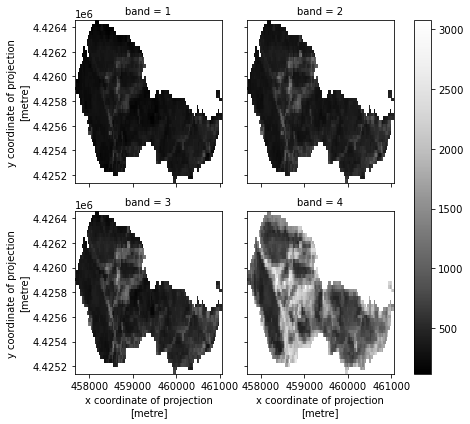
# Plot the final stacked data
post_fire_stack.plot.imshow(col="band",
                            col_wrap=2,
                            cmap="Greys_r")
plt.show()
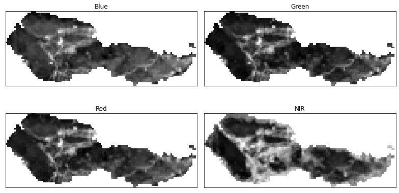
Plot Data Using EarthPy
To save some code, you can plot with earthpy instead. Earthpy
will clean up your plot for you a bit, saving the steps of cleaning up axes
and adding titles.
# Plot using earthpy
band_titles = ["Blue",
               "Green",
               "Red",
               "NIR"]

ep.plot_bands(post_fire_stack,
              figsize=(11, 6),
              cols=2,
              title=band_titles,
              cbar=False)
plt.show()
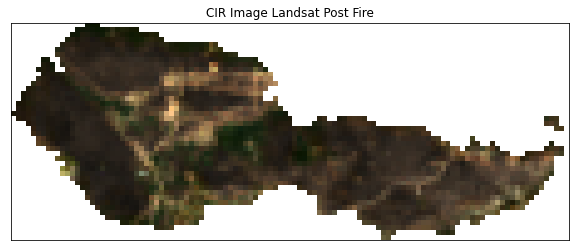
Create an RGB Plot of Your Landsat Raster Data
If you want to plot your data as a color composit RGB map, you can use earthpy’s
plot_rgb() function.
# Plot array
ep.plot_rgb(post_fire_stack,
            rgb=[2, 1, 0],
            title="CIR Image Landsat Post Fire")

plt.show()
def process_bands(paths, crop_layer, stack=False):
    """
    Open, clean and crop a list of raster files using rioxarray.

    Parameters
    ----------
    paths : list
        A list of paths to raster files that could be stacked (of the same
        resolution, crs and spatial extent).

    crop_layer : geodataframe
        A geodataframe containing the crop geometry that you wish to crop your
        data to.

    stack : boolean
        If True, return a stacked xarray object. If false will return a list
        of xarray objects.

    Returns
    -------
        Either a list of xarray objects or a stacked xarray object
    """

    all_bands = []
    for i, aband in enumerate(paths):
        cleaned = open_clean_band(aband, crop_layer)
        cleaned["band"] = i+1
        all_bands.append(cleaned)

    if stack:
        print("I'm stacking your data now.")
        return xr.concat(all_bands, dim="band")
    else:
        print("Returning a list of xarray objects.")
        return all_bands
# Open up boundary extent using GeoPandas
fire_boundary_path = os.path.join("cold-springs-fire",
                                  "vector_layers",
                                  "fire-boundary-geomac",
                                  "co_cold_springs_20160711_2200_dd83.shp")

fire_boundary = gpd.read_file(fire_boundary_path)

# Get a list of required bands - bands 2 through 5
all_landsat_post_bands = glob(os.path.join(landsat_post_fire_path,
                                           "*band[2-5]*.tif"))
all_landsat_post_bands.sort()

# Get CRS of landsat data and reproject fire boundary
landsat_crs = es.crs_check(all_landsat_post_bands[0])
fire_boundary_utmz13 = fire_boundary.to_crs(landsat_crs)
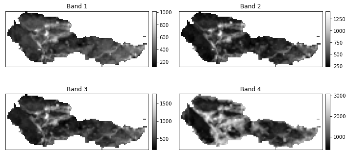
# Process all bands
post_fire_stack = process_bands(all_landsat_post_bands,
                                fire_boundary_utmz13,
                                stack=True)
post_fire_stack.shape
I'm stacking your data now.
(4, 44, 113)
# Plot using earthpy
band_titles = ["Blue Band",
               "Green Band",
               "Red Band",
               "NIR Band"]

# Plot the final data
ep.plot_bands(post_fire_stack,
             cols=2,
             figsize=(10,5))
plt.suptitle("Cleaned and Cropped Landsat Bands")
plt.show()
<Figure size 432x288 with 0 Axes>
Share on
Twitter Facebook Google+ LinkedIn
Leave a Comment