Lesson 2. GIS in Python: Reproject Vector Data.
Learning Objectives
- Identify the CRS of a spatial dataset and reproject it to another CRS in Python.
- Clip a spatial vector point and line layer to the spatial extent of a polygon layer in Python using geopandas.
- Dissolve polygons based upon an attribute in Python using geopandas.
- Join spatial attributes from one shapefile to another in Python using geopandas.
Data in Different Coordinate Reference Systems
In the previous chapter, you attempted to plot two datasets together - a roads layer and the locations of plots where our field work was occuring. The layers did not plot properly even though you know the data are for the same geographic location. The challenge as a reminder is below:
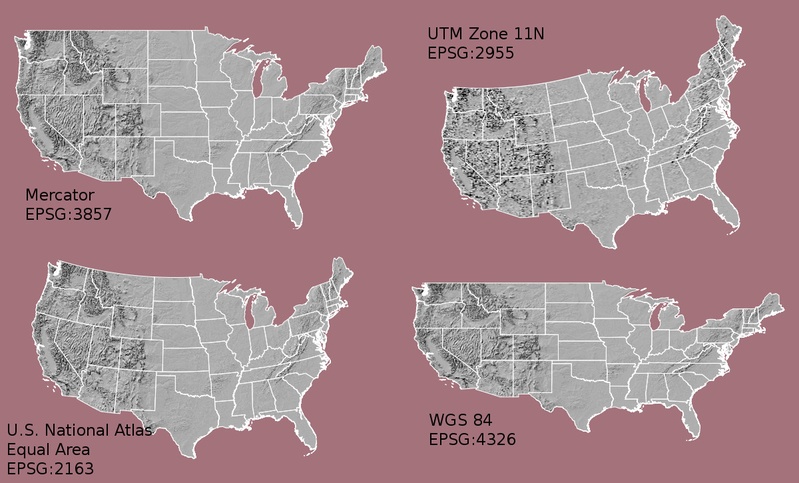
Often when data do not line up properly, it is because they are in different coordinate reference systems (CRS). In this lesson you will learn how to reproject data from one CRS to another - so that the data line up properly.
Working With Spatial Data From Different Sources
You often need to gather spatial datasets for from different sources and/or data that cover different spatial extents. Spatial data from different sources and that cover different extents are often in different Coordinate Reference Systems (CRS).
Some reasons for data being in different CRSs include:
- The data are stored in a particular CRS convention used by the data provider which might be a federal agency, or a state planning office.
- The data are stored in a particular CRS that is customized to a region. For instance, many states prefer to use a State Plane projection customized for that state.
import os
import numpy as np
import matplotlib.pyplot as plt
import seaborn as sns
import geopandas as gpd
import earthpy as et

# Setting plotting style for the notebook
sns.set_style("white")
sns.set(font_scale=1.5)

# Set working dir & get data
data = et.data.get_data('spatial-vector-lidar')
os.chdir(os.path.join(et.io.HOME, 'earth-analytics'))
Revisiting the challenge from a previous lesson, here are the two layers: Notice the CRS of each layer.
# Import the data
sjer_roads_path = os.path.join("data", "spatial-vector-lidar", "california",
                               "madera-county-roads", "tl_2013_06039_roads.shp")
sjer_roads = gpd.read_file(sjer_roads_path)

# aoi stands for area of interest
sjer_aoi_path = os.path.join("data", "spatial-vector-lidar", "california",
                             "neon-sjer-site", "vector_data", "SJER_crop.shp")
sjer_aoi = gpd.read_file(sjer_aoi_path)

# View the Coordinate Reference System of both layers
print(sjer_roads.crs)
print(sjer_aoi.crs)
epsg:4269
epsg:32611
To plot the data together, they need to be in the same CRS. You can change the CRS which means you are reproject the data from one CRS to another CRS using the geopandas method:
to_crs(specify-crs-here)
The CRS can be specified using an epsg code - as follows:
epsg=4269
IMPORTANT: When you reproject data you are modifying it. Thus you are introducing some uncertainty into your data. While this is a slightly less important issue when working with vector data (compared to raster), it’s important to consider.
Often you may consider keeping the data that you are doing the analysis on in the correct projection that best relates spatially to the area that you are working in. IE use the CRS that best minimizes errors in distance/ area etc based on your analysis.
If you are simply reprojecting to create a base map then it doesn’t matter what you reproject!
# Reproject the aoi to match the roads layer
sjer_aoi_wgs84  = sjer_aoi.to_crs(epsg=4269)
# Plot the data
fig, ax = plt.subplots(figsize=(12, 8))

sjer_roads.plot(cmap='Greys', ax=ax, alpha=.5)
sjer_aoi_wgs84.plot(ax=ax, markersize=10, color='r')

ax.set_title("Madera County Roads with SJER AOI");
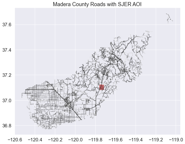
Great! you’ve now reprojected a dataset to be able to map the sjer AOI on top of the roads layer. Let’s try this process again but this time using some census data boundaries.
Import US Boundaries - Census Data
There are many good sources of boundary base layers that you can use to create a basemap. Some Python packages even have these base layers built in to support quick and efficient mapping. In this tutorial, you will use boundary layers for the United States, provided by the United States Census Bureau.
It is useful to have shapefiles to work with because you can add additional attributes to them if need be - for project specific mapping.
Read US Boundary File
You will use the geopandas .read_file() function to import the /usa-boundary-layers/US-State-Boundaries-Census-2014 layer into Python. This layer contains the boundaries of all continental states in the U.S. Please note that these data have been modified and reprojected from the original data downloaded from the Census website to support the learning goals of this tutorial.
# Import data into geopandas dataframe
state_boundary_us_path = os.path.join("data", "spatial-vector-lidar",
                                      "usa", "usa-states-census-2014.shp")
state_boundary_us = gpd.read_file(state_boundary_us_path)

# View data structure
type(state_boundary_us)
geopandas.geodataframe.GeoDataFrame
# View the first few lines of the data
state_boundary_us.head()
| STATEFP | STATENS | AFFGEOID | GEOID | STUSPS | NAME | LSAD | ALAND | AWATER | region | geometry | |
|---|---|---|---|---|---|---|---|---|---|---|---|
| 0 | 06 | 01779778 | 0400000US06 | 06 | CA | California | 00 | 403483823181 | 20483271881 | West | MULTIPOLYGON Z (((-118.59397 33.46720 0.00000,... |
| 1 | 11 | 01702382 | 0400000US11 | 11 | DC | District of Columbia | 00 | 158350578 | 18633500 | Northeast | POLYGON Z ((-77.11976 38.93434 0.00000, -77.04... |
| 2 | 12 | 00294478 | 0400000US12 | 12 | FL | Florida | 00 | 138903200855 | 31407883551 | Southeast | MULTIPOLYGON Z (((-81.81169 24.56874 0.00000, ... |
| 3 | 13 | 01705317 | 0400000US13 | 13 | GA | Georgia | 00 | 148963503399 | 4947080103 | Southeast | POLYGON Z ((-85.60516 34.98468 0.00000, -85.47... |
| 4 | 16 | 01779783 | 0400000US16 | 16 | ID | Idaho | 00 | 214045425549 | 2397728105 | West | POLYGON Z ((-117.24303 44.39097 0.00000, -117.... |
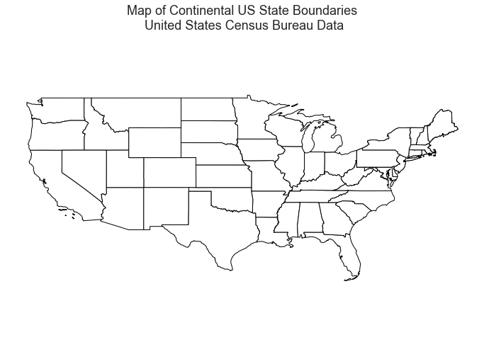
Next, plot the U.S. states data. Below you use geopandas to plot your geodataframe. Also notice that you are using ax.set_axis_off() to hide the x, y axis of our plot.
# Plot the data
fig, ax = plt.subplots(figsize = (12,8))
state_boundary_us.plot(ax = ax, facecolor = 'white', edgecolor = 'black')

# Add title to map
ax.set(title="Map of Continental US State Boundaries\n United States Census Bureau Data")

# Turn off the axis
plt.axis('equal')
ax.set_axis_off()

plt.show()
U.S. Boundary Layer
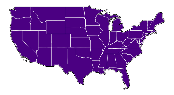
You can add a boundary layer of the United States to your map to make it look nicer. You will import data/week5/usa-boundary-layers/US-Boundary-Dissolved-States. If you specify a thicker line width using linewidth=4 for the border layer, it will make our map visually pop!
# Import United States country boundary data
county_boundary_us_path = os.path.join("data", "spatial-vector-lidar",
                                       "usa", "usa-boundary-dissolved.shp")
country_boundary_us = gpd.read_file(county_boundary_us_path)

type(country_boundary_us)
geopandas.geodataframe.GeoDataFrame
# Plot data
fig, ax = plt.subplots(figsize = (12,7))
country_boundary_us.plot(ax=ax,
                         alpha=1,
                         edgecolor="black",
                         color = "white",
                         linewidth=4)

state_boundary_us.plot(ax = ax,
                      color = "indigo",
                      edgecolor = "white",
                      linewidth = 1)
ax.set_axis_off()
plt.show()
Next, add the SJER study area site locations to your map. As you add these layers, take note of the class of each object and the CRS.
HINT: AOI stands for “Area of Interest”. This is your study area.
# Plot the data
fig, ax = plt.subplots(figsize = (6,6))

sjer_aoi.plot(ax=ax, color = "indigo")
ax.set(title='San Joachin Experimental Range \n Area of interest (AOI)')

ax.set_axis_off()
plt.show()

The SJER AOI layer plots nicely. Next, add it as a layer on top of the U.S. states and boundary layers in your basemap plot.
fig, ax = plt.subplots(figsize=(6, 6))

country_boundary_us.plot(ax=ax,
                         edgecolor="black",
                         color = "white",
                         linewidth=3,
                         alpha=.8)

state_boundary_us.plot(ax = ax,
                       color = "white",
                       edgecolor ="gray")
sjer_aoi.plot(ax=ax, color = "indigo")

# Turn off axis
ax.set_axis_off()
plt.show()

What do you notice about the resultant plot? Do you see the AOI boundary in the California area? Is something wrong with our map?
Let’s check out the CRS (.crs) of both datasets to see if you can identify any issues that might cause the point location to not plot properly on top of our U.S. boundary layers.
# View CRS of each layer
print(sjer_aoi.crs)
print(country_boundary_us.crs)
print(state_boundary_us.crs)
epsg:32611
epsg:4326
epsg:4326
Looking at the CRS information returned above, it seems as if our data are in different CRS’. You can tell this by looking at the EPSG codes:
- 32611
- 4326
Optional challenge
Look up the EPSG codes listed above on the spatialreference.org website and answer the following questions.
- What CRS does each code correspond with?
- Is the CRS projected or geographic?
CRS Units - View Object Extent
Next, let’s view the extent or spatial coverage for the sjer_aoi spatial object compared to the state_boundary_us object.
# View spatial extent for both layers
print(sjer_aoi.total_bounds)
print(state_boundary_us.total_bounds)
[ 254570.567      4107303.07684455  258867.40933092 4112361.92026107]
[-124.725839   24.498131  -66.949895   49.384358]
Note the difference in the units for each object. The extent for state_boundary_us is in latitude and longitude which yields smaller numbers representing decimal degree units. Our AOI boundary point is in UTM, is represented in meters.
Most importantly the two extents DO NOT OVERLAP. Yet you know that your data should overlap.
Reproject Vector Data
Now you know your data are in different CRS. To address this, you have to modify or reproject the data so they are all in the same CRS. You can use .to_crs() function to reproject your data. When you reproject the data, you specify the CRS that you wish to transform your data to. This CRS contains the datum, units and other information that Python needs to reproject our data.
The to_crs() function requires two inputs:
- the name of the object that you wish to transform
- the CRS that you wish to transform that object to - - this can be in EPSG format or an entire project 4 string. In this case you can use the
crsvalue from thestate_boundary_usobject :.to_crs(state_boundary_us.crs)
Data Tip: .to_crs() will only work if your original spatial object has a CRS assigned to it AND if that CRS is the correct CRS!
Next, let’s reproject our point layer into the geographic - latitude and longitude WGS84 coordinate reference system (CRS).
# Reproject the aoi to the same CRS as the state_boundary_use object
sjer_aoi_WGS84 = sjer_aoi.to_crs(state_boundary_us.crs)

# View CRS of new reprojected layer
print(sjer_aoi.total_bounds)
print('sjer_aoi crs: ', sjer_aoi_WGS84.crs)
print('state boundary crs:', state_boundary_us.crs)
[ 254570.567      4107303.07684455  258867.40933092 4112361.92026107]
sjer_aoi crs:  epsg:4326
state boundary crs: epsg:4326
If you want, you can reproject using the full proj.4 string too. Below, the CRS for the EPSG code 4326 from the spatialreference.org website is used as the crs argument.
# Reproject using the full proj.4 string copied from spatial reference.org
sjer_aoi_WGS84_2 = sjer_aoi.to_crs("+proj=longlat +ellps=WGS84 +datum=WGS84 +no_defs")
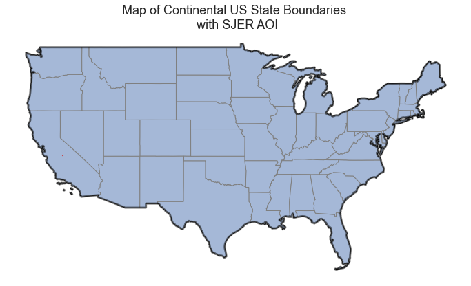
Once our data are reprojected, you can try to plot again.
fig, ax = plt.subplots(figsize = (12,8))

state_boundary_us.plot(ax = ax,
                      linewidth=1,
                      edgecolor="black")

country_boundary_us.plot(ax=ax,
                         alpha=.5,
                         edgecolor="black",
                         color = "white",
                         linewidth=3)
sjer_aoi_WGS84.plot(ax=ax,
                    color='springgreen',
                   edgecolor = "r")

ax.set(title="Map of Continental US State Boundaries \n with SJER AOI")

ax.set_axis_off()
plt.show()
It’s hard to see the tiny extent box on a map of the entire US. Try to zoom in on just a small portion of the map to better see the extent. To do this you can adjust the x and y limits as follows:
ax.set(xlim=[minx, maxx], ylim=[miny, maxy])
# Zoom in on just the area
fig, ax = plt.subplots(figsize = (12,8))

state_boundary_us.plot(ax = ax,
                      linewidth=1,
                      edgecolor="black")

country_boundary_us.plot(ax=ax,
                         alpha=.5,
                         edgecolor="black",
                         color = "white",
                         linewidth=3)

sjer_aoi_WGS84.plot(ax=ax,
                    color='springgreen',
                   edgecolor = "r")

ax.set(title="Map of Continental US State Boundaries \n with SJER AOI")
ax.set(xlim=[-125, -116], ylim=[35, 40])

# Turn off axis
ax.set(xticks = [], yticks = []);
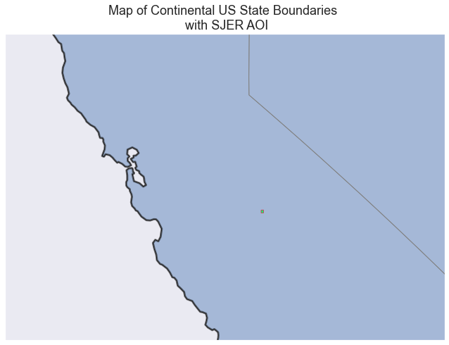
Great! The plot worked this time however now, the AOI boundary is a polygon and it’s too small to see on the map. Let’s convert the polygon to a polygon CENTROID (a point) and plot again. If your data are represented as a point you can change the point size to make it more visible.
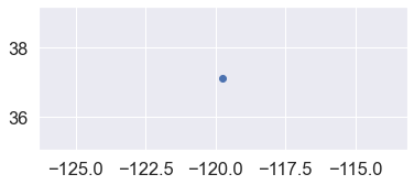
To do this, you’ll access the centroid attribute of your AOI polygon using .centroid.
# Grab the centroid x, y location of the aoi and turn it into a new spatial object.
AOI_point = sjer_aoi_WGS84["geometry"].centroid
type(AOI_point)
<ipython-input-19-2d86642bd8b9>:2: UserWarning: Geometry is in a geographic CRS. Results from 'centroid' are likely incorrect. Use 'GeoSeries.to_crs()' to re-project geometries to a projected CRS before this operation.

  AOI_point = sjer_aoi_WGS84["geometry"].centroid
geopandas.geoseries.GeoSeries
sjer_aoi_WGS84["geometry"].centroid.plot();
<ipython-input-20-2742f90a2820>:1: UserWarning: Geometry is in a geographic CRS. Results from 'centroid' are likely incorrect. Use 'GeoSeries.to_crs()' to re-project geometries to a projected CRS before this operation.

  sjer_aoi_WGS84["geometry"].centroid.plot();
fig, ax = plt.subplots(figsize = (12,7))

state_boundary_us.plot(ax = ax,
                      linewidth=1,
                      edgecolor="black")

country_boundary_us.plot(ax=ax,
                         alpha=.7,
                         edgecolor="black",
                         color = "white",
                         linewidth=3)

AOI_point.plot(ax=ax,
              markersize=80,
              color='purple',
              marker='*')

ax.set(title="Map of Continental US State Boundaries \n with SJER AOI")

# Turn off axis
ax.set_axis_off();
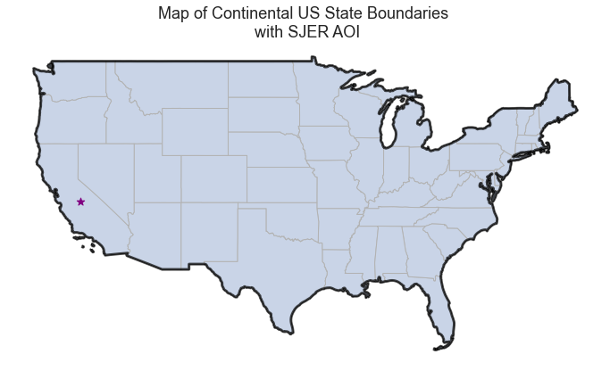
Reprojecting our data ensured that things line up on our map! It will also allow us to perform any required geoprocessing (spatial calculations / transformations) on our data.
Additional Resources - CRS
Share on
Twitter Facebook Google+ LinkedIn
Leave a Comment