Lesson 3. Activity: Plot Spatial Raster Data in Python
Learning Objectives
- Apply your skills in plotting spatial raster data using open source Python.
Plot Spatial Data in Python
Throughout these chapters, one of the main focuses has been opening, modifying, and plotting all forms of spatial data. The chapters have covered a wide array of these types of data, including all types of vector data, elevation data, imagery data, and more! You’ve used a combination of multiple libraries to open and plot spatial data, including pandas, geopandas, matplotlib, earthpy, and various others. Often earth analytics will combine vector and raster data to do more meaningful analysis on a research question. Plotting these various types of data together can be challenging, but also very informative.
Challenge Your Skills
In this challenge you will be asked to use the appropriate packages and tools to plot each type of spatial data that have been covered so far. First, you will plot out various forms of vector data, then raster data, and finally you will plot a combination of the raster and vector data.
# Import Packages

import os
from glob import glob
import matplotlib.pyplot as plt
import seaborn as sns
import pandas as pd
import geopandas as gpd
import rioxarray as rxr
from rasterio.plot import plotting_extent
import folium
import earthpy as et
import earthpy.plot as ep
import earthpy.spatial as es

import warnings
warnings.filterwarnings('ignore', 'GeoSeries.notna', UserWarning)

# Add seaborn general plot specifications
sns.set(font_scale=1.5, style="whitegrid")
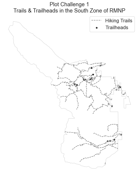
Challenge 1: Create a Map Of RMNP Trails for the South Zone of the Park
The first plot you are going to make is a vector plot that displays hiking trails in Rocky Mountain National Park (RMNP) - which is located in Colorado.
To make this plot, do the following:
- Read in the trails, trailsheads and ranger zones data for the Rocky Mountain National Park trails and the National Parks Service boundaries. The code to open the data is in the cell below for you to run.
- Create a new GeoDataFrame that only contains the South Zone of the RMNP ranger zones
ranger_zones[ranger_zones["SUBDISTRIC"] == ["SOUTH"]data for the park. - Change the Coordinate Reference System of the boundary dataset to match the trails dataset. To get the Coordinate Reference System of the trails dataset, you can use
trails_dataframe_name.crs. To set it to the boundary dataset, you can use theto_crs()function like so:south_zone_boundary_geodataframe_name.to_crs(trails_dataframe_name.crs) - Plot the trails data and the trailheads data together in a map.
- Add the polygon boundary of the South Ranger zone to the map.
- Change the symbology for the lines and points on the map. For lines, you will change the
linestyle=argument options for this argument here and for points you will modify themarker=arguement options for this argument here. - We want a legend for this map, to show the symbology of trails and trail heads. To create this, in the plotting functions for your GeoDataFrames, add an argument
label=and set it to what you want to call the trails and trailheads on your maps. Also, make sure you have the following lines of code in your plot. It will grab the labels you set in the plot functions and add them to the legend.handles, labels = ax.get_legend_handles_labels() ax.legend(handles, labels) - Add a title to your plot.
Your plot should look similar to the plot below.
Data Tip:
# Open RMNP Boundary -- we might not need this
# RMNP Boundary Layer: Lat lon 4326 -- direct download
rmnp_boundary = gpd.read_file(
    "https://opendata.arcgis.com/datasets/7cb5f22df8c44900a9f6632adb5f96a5_0.geojson")
# Trails are UTM Zone 13N --  reproject to lat long
rmnp_trails = gpd.read_file(
    "https://opendata.arcgis.com/datasets/e1e0bcb87eb94960bc04f76e03936385_0.geojson")
rmnp_trails_4326 = rmnp_trails.to_crs(rmnp_boundary.crs)
# Open ranger zones  - EPSG 4326
ranger_zones = gpd.read_file(
    "https://opendata.arcgis.com/datasets/fdffd3272ba546da9176416b814d2e8f_0.geojson")

# Trailheads - 4326
trailheads = gpd.read_file(
    "https://opendata.arcgis.com/datasets/55748f2f1d8a4db7aa26f7549e74be57_0.geojson")
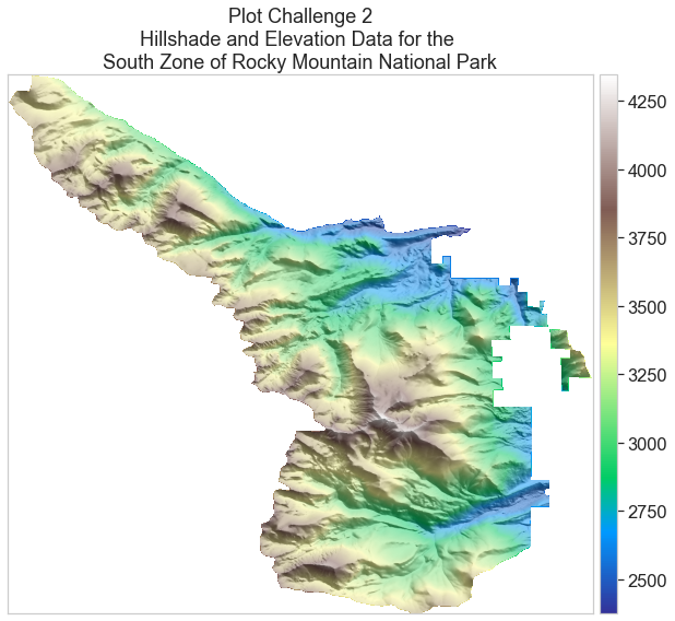
Challenge 2: Overlay a Terrain Model on top of a Hillshade
Next you will create a base map to put your trails on. In order to do this, you will use a Digital Elevation Model (USGS_1_n41w106.tif) for RMNP. The code to download the DEM is in the cell below. Once that is downloaded, you must complete the following steps to create the hillshade and plot the two rasters on top of each other.
- Read in the USGS DEM with rioxarray.
- Clip the data to the extent of the south zone boundary you plotted earlier using rioxarray and the geometry of the boundary.
- Create a hillshade from the clipped DEM using the syntax:
es.hillshade(clipped_data[0]). This function outputs a numpy array with the hillshade data. - Overlay the clipped DEM array on top of the hillshade array you just created.
- Be sure to add a title to your plot.
Your plot should look similar to the plot below.
# All these data are 4326 so reprojecting to that above makes sense
et.data.get_data(url="https://ndownloader.figshare.com/files/23399609")
os.chdir(os.path.join(et.io.HOME, "earth-analytics", "data"))
ned_30m_path = os.path.join("earthpy-downloads", "USGS_1_n41w106.tif")
Downloading from https://ndownloader.figshare.com/files/23399609
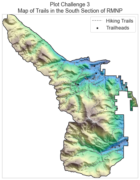
Challenge 3: Overlay Trails on top of Elevation Data.
Next you will overlay the trails data on top of the elevation data that you plotted above. Keep in mind a few things when you do this
- You will need to create a plotting_extent object to use in the
extent=plot parameter inep.plot_bands()to ensure that your raster data line up with the vector data. Make sure you use the data and metadata that was the output of your clip to create the plotting_extent object so that the extent is correct. Your code should look like the following:ned_cl_extent = plotting_extent(clipped_data[0], clipped_data.rio.transform()) - The legibility of data will change with the background data, so be sure to adjust colors/thickness of your data if you need to in order to make it visible.
- Be sure to add a title to your map.
Your plot should look similar to the plot below.
Data Tip: If plotting extents are causing you trouble, this lesson covering plotting extents may help you.
Challenge 4: OPTIONAL Plot Interactive Vector Data
Below is a map that was made with folium to create an interactive map of the trails and trailheads in Rocky Mountain National Park. This is another way to give your data a background to give it context, besides using elevation or imagery data. Notice you can zoom in/out and move around the map by clicking and dragging. However, there are some aspects that you can change to make the map better! Here are some improvements you can give to the map:
- You can see where the lines are assigned colors with the
styledictionary. Change the color to an easier color to see, as the green blends in with the background. - The play icon is a nice marker for trailheads, but not the only option. Change the
icon=argument infolium.Icon()to be another shape. There’s a list of usable icons here. Note: Not all of the icons on that site will work, so if you pick one and it doesn’t display try a different option! - When you click on the trailhead points, you will see it displays the
GEOMETRYIDvalue for the point. It may be more useful to display thePOINAMEcolumn, which has the trail name stored in it. Change the column to the correct name so it displays properly. - You may notice that the map initially starts really zoomed out. Change the
zoom_startto make the map start close to the coverage of the data.
# Style Dictionary
style = {'color': 'green'}

# Adding the lines to the map
trails_south_json = trails_south.to_json()
interactive_map = folium.Map(location=[40.37244, -105.66472],
                             zoom_start=7)
lines = folium.features.GeoJson(trails_south_json,
                                style_function=lambda x: style)
interactive_map.add_child(lines)

# Adding the points to the map
for i in range(len(trailheads_south)):
    folium.Marker([trailheads_south.iloc[i].geometry.y, trailheads_south.iloc[i].geometry.x],
                  popup=trailheads_south.iloc[i]['GEOMETRYID'],
                  icon=folium.Icon(icon='play')).add_to(interactive_map)
interactive_map
Share on
Twitter Facebook Google+ LinkedIn
Leave a Comment