Lesson 3. Introduction to Spatial Vector Data File Formats in Open Source Python
Fundamentals of Vector Data in Python
In this lesson, you will be introduced to the spatial vector data structure
and the shapefile file format (.shp). You will also learn how to open, explore and plot
vector data using the Geopandas package in Python.
Learning Objectives
After completing this lesson, you will be able to:
- Describe the characteristics of 3 key vector data structures: points, lines and polygons.
- Open a shapefile in Python using Geopandas -
gpd.read_file(). - Plot a shapfile in Python using Geopandas -
gpd.plot().
Recommended Readings
This lesson is an introduction to working with spatial data. If you wish to dive more deeply into working with spatial data, check out the intermediate earth data science textbook chapter on spatial vector data.
About Spatial Vector Data
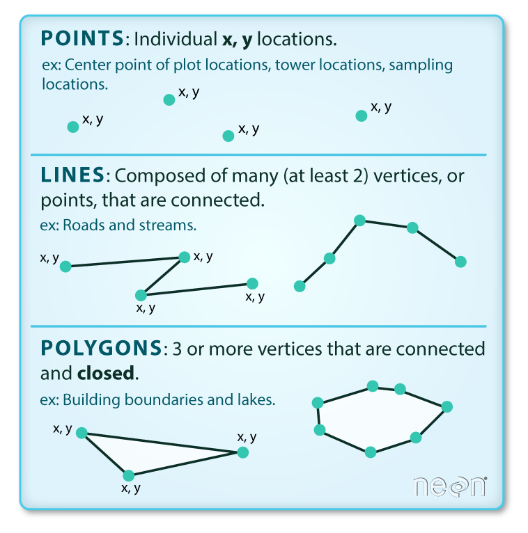
Vector data are composed of discrete geometric locations (x, y values) known as vertices that define the “shape” of the spatial object. The organization of the vertices determines the type of vector that you are working with. There are three types of vector data:
-
Points: Each individual point is defined by a single x, y coordinate. Examples of point data include: sampling locations, the location of individual trees or the location of plots.
-
Lines: Lines are composed of many (at least 2) vertices, or points, that are connected. For instance, a road or a stream may be represented by a line. This line is composed of a series of segments, each “bend” in the road or stream represents a vertex that has defined
x, ylocation. -
Polygons: A polygon consists of 3 or more vertices that are connected and “closed”. Thus, the outlines of plot boundaries, lakes, oceans, and states or countries are often represented by polygons.
Introduction to the Shapefile File Format Which Stores Points, Lines, and Polygons
Geospatial data in vector format are often stored in a shapefile
format (.shp). Because the structure of points, lines, and polygons are
different, each individual shapefile can only contain one vector
type (all points, all lines or all polygons). You will not find
a mixture of point, line and polygon objects in a single shapefile.
Objects stored in a shapefile often have a set of associated
attributes that describe the data. For example, a line
shapefile that contains the locations of streams might also
contain the associated stream name, stream “order” and other
information about each stream line object.
Data Tip: More about shapefiles can found on Wikipedia.
GeoJSON Files and Other Vector Formats
The shapefile is not the only way that vector data are stored. Geospatial data can also be delivered in a GeoJSON format, or even a tabular format where the spatial information is contained in columns.
What Data Are Stored In Spatial Vector Formats?
Some examples of data that often are provided in a vector format include:
- census data including municipal boundaries
- roads, powerlines and other infrastructure boundaries
- political boundaries
- building outlines
- water bodies and river systems
- ecological boundaries
- city locations
- object locations including plots, stream gages, and building locations
Import Shapefile Data Into Python Using Geopandas
You will use the geopandas library to work with vector data in
Python. Geopandas is built on top of the Python Pandas library.
It stores spatial data in a tabular, dataframe format.
# Import packages
import os

import matplotlib.pyplot as plt
import geopandas as gpd
import earthpy as et
To begin, set your working directory to earth-analytics and then download a
single shapefile. You will start with working with the Natural Earth
country boundary lines layer.
Data Tip: Note that below you are using EarthPy to download a dataset from naturalearthdata.com. EarthPy creates the earth-analytics directory for you when you use it. You set the working directory after you download the data as a precaution to ensure that the earth-analytics directory already exists on your computer. This is not a standard order of operations but we are demonstrating it here to ensure the notebook runs on all computers!
# Download the data and set working directory
et.data.get_data(
    url='https://www.naturalearthdata.com/http//www.naturalearthdata.com/download/50m/cultural/ne_50m_admin_0_boundary_lines_land.zip')

# Set working directory - earthpy creates earth-analytics for you in your home dir
os.chdir(os.path.join(et.io.HOME, 'earth-analytics'))
Downloading from https://www.naturalearthdata.com/http//www.naturalearthdata.com/download/50m/cultural/ne_50m_admin_0_boundary_lines_land.zip
Extracted output to /root/earth-analytics/data/earthpy-downloads/ne_50m_admin_0_boundary_lines_land
Next, you open the data using Geopandas. You can view the first 5 rows of the
data using .head() in the same way you used .head() for Pandas dataframes.
coastlines_url = "https://www.naturalearthdata.com/http//www.naturalearthdata.com/download/50m/physical/ne_50m_coastline.zip"

et.data.get_data(url=coastlines_url)

coastlines_path = os.path.join("data", "earthpy-downloads",
                               "ne_50m_coastline",
                               "ne_50m_coastline.shp")

coastlines = gpd.read_file(coastlines_path)
coastlines.head()
Downloading from https://www.naturalearthdata.com/http//www.naturalearthdata.com/download/50m/physical/ne_50m_coastline.zip
Extracted output to /root/earth-analytics/data/earthpy-downloads/ne_50m_coastline
| scalerank | featurecla | min_zoom | geometry | |
|---|---|---|---|---|
| 0 | 0 | Coastline | 1.5 | LINESTRING (180.00000 -16.15293, 179.84814 -16... |
| 1 | 0 | Coastline | 4.0 | LINESTRING (177.25752 -17.05420, 177.28740 -17... |
| 2 | 0 | Coastline | 4.0 | LINESTRING (127.37266 0.79131, 127.35381 0.847... |
| 3 | 0 | Coastline | 3.0 | LINESTRING (-81.32231 24.68506, -81.42007 24.7... |
| 4 | 0 | Coastline | 4.0 | LINESTRING (-80.79941 24.84629, -80.83887 24.8... |
GeoPandas Creates GeoDataFrames Which Have the Same Structure As Pandas DataFrames
The structure of a Geopandas GeoDataFrame is very similar to a
Pandas dataframe. A few differences include:
- the
GeoDataFramecontains a geometry column which stores spatial information. The geometry column in yourGeoDataFramestores the boundary information (the lines that make up each shape in your data). This allows you to plot points, lines or polygons. - the
GeoDataFramestores spatial attributes such as coordinate reference systems and spatial extents.
Similar to Pandas, you can plot the data using .plot()
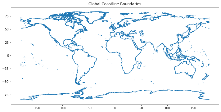
# Plot the data
f, ax1 = plt.subplots(figsize=(12, 6))
coastlines.plot(ax=ax1)

# Add a title to your plot
ax1.set(title="Global Coastline Boundaries")
plt.show()
Check the Spatial Vector Data Type
You can look at the data to figure out what type of data are stored in the
shapefile (points, line or polygons). However, you can also get that information
by calling .geom_type
# Is the geometry type point, line or polygon?
coastlines.geom_type
0       LineString
1       LineString
2       LineString
3       LineString
4       LineString
           ...
1423    LineString
1424    LineString
1425    LineString
1426    LineString
1427    LineString
Length: 1428, dtype: object
Also similar to Pandas, you can view descriptive information about the
GeoDataFrame using .info(). This includes the number of columns, rows
and the header name and type of each column.
coastlines.info()
<class 'geopandas.geodataframe.GeoDataFrame'>
RangeIndex: 1428 entries, 0 to 1427
Data columns (total 4 columns):
 #   Column      Non-Null Count  Dtype
---  ------      --------------  -----
 0   scalerank   1428 non-null   int64
 1   featurecla  1428 non-null   object
 2   min_zoom    1428 non-null   float64
 3   geometry    1428 non-null   geometry
dtypes: float64(1), geometry(1), int64(1), object(1)
memory usage: 44.8+ KB
Open Vector Point Data
Next, you will open up another shapefile using Geopandas.
# Open a second layer
et.data.get_data(
    url='https://www.naturalearthdata.com/http//www.naturalearthdata.com/download/50m/cultural/ne_50m_populated_places_simple.zip')

# Create a path to the populated places shapefile
populated_places_path = os.path.join("data", "earthpy-downloads",
                                     "ne_50m_populated_places_simple",
                                     "ne_50m_populated_places_simple.shp")

cities = gpd.read_file(populated_places_path)
cities.head()
Downloading from https://www.naturalearthdata.com/http//www.naturalearthdata.com/download/50m/cultural/ne_50m_populated_places_simple.zip
Extracted output to /root/earth-analytics/data/earthpy-downloads/ne_50m_populated_places_simple
| scalerank | natscale | labelrank | featurecla | name | namepar | namealt | diffascii | nameascii | adm0cap | ... | rank_max | rank_min | geonameid | meganame | ls_name | ls_match | checkme | min_zoom | ne_id | geometry | |
|---|---|---|---|---|---|---|---|---|---|---|---|---|---|---|---|---|---|---|---|---|---|
| 0 | 10 | 1 | 5 | Admin-1 region capital | Bombo | None | None | 0 | Bombo | 0.0 | ... | 8 | 7 | 0.0 | None | None | 0 | 0 | 7.0 | 1159113923 | POINT (32.53330 0.58330) |
| 1 | 10 | 1 | 5 | Admin-1 region capital | Fort Portal | None | None | 0 | Fort Portal | 0.0 | ... | 7 | 7 | 233476.0 | None | None | 0 | 0 | 7.0 | 1159113959 | POINT (30.27500 0.67100) |
| 2 | 10 | 1 | 3 | Admin-1 region capital | Potenza | None | None | 0 | Potenza | 0.0 | ... | 8 | 8 | 3170027.0 | None | None | 0 | 0 | 7.0 | 1159117259 | POINT (15.79900 40.64200) |
| 3 | 10 | 1 | 3 | Admin-1 region capital | Campobasso | None | None | 0 | Campobasso | 0.0 | ... | 8 | 8 | 3180991.0 | None | None | 0 | 0 | 7.0 | 1159117283 | POINT (14.65600 41.56300) |
| 4 | 10 | 1 | 3 | Admin-1 region capital | Aosta | None | None | 0 | Aosta | 0.0 | ... | 7 | 7 | 3182997.0 | None | None | 0 | 0 | 7.0 | 1159117361 | POINT (7.31500 45.73700) |
5 rows × 39 columns
Challenge 1: What Geometry Type Are Your Data
Check the geometry type of the cities object that you opened above in your code.
0       Point
1       Point
2       Point
3       Point
4       Point
        ...
1244    Point
1245    Point
1246    Point
1247    Point
1248    Point
Length: 1249, dtype: object
Creating Maps Using Multiple Shapefiles
You can create maps using multiple shapefiles with Geopandas in a similar way that you may do so using a graphical user interface (GUI) tool like ArcGIS or QGIS (open source alternative to ArcGIS). To do this you will need to open a second spatial file. Below you will use the Natural Earth populated places shapefile to add additional layers to your map.
To plot two datasets together, you will first create a Matplotlib figure object.
Notice in the example below that you define the figure ax1 in the first line.
You then tell GeoPandas to plot the data on that particular figure using the
parameter ax=
The code looks like this:
boundary_lines.plot(ax=ax1)
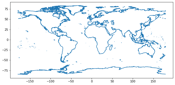
f, ax1 = plt.subplots(figsize=(10, 6))
coastlines.plot(ax=ax1)
plt.show()
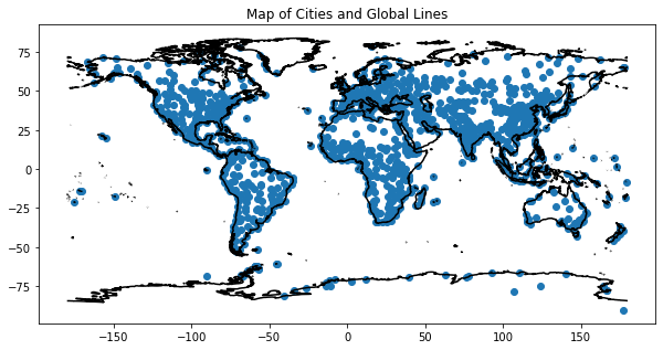
To add another layer to your map, you can add a second .plot() call and
specify the ax= to be ax1 again. This tells Python to layer the two
datasets in the same figure.
# Create a map or plot with two data layers
f, ax1 = plt.subplots(figsize=(10, 6))
coastlines.plot(ax=ax1,
                color="black")
cities.plot(ax=ax1)

# Add a title
ax1.set(title="Map of Cities and Global Lines")
plt.show()
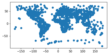
If you don’t specify the axis when you plot using ax=, each layer will be plotted on a
separate figure! See the example below.
f, ax1 = plt.subplots(figsize=(10, 6))
coastlines.plot(ax=ax1)
cities.plot()
plt.show()

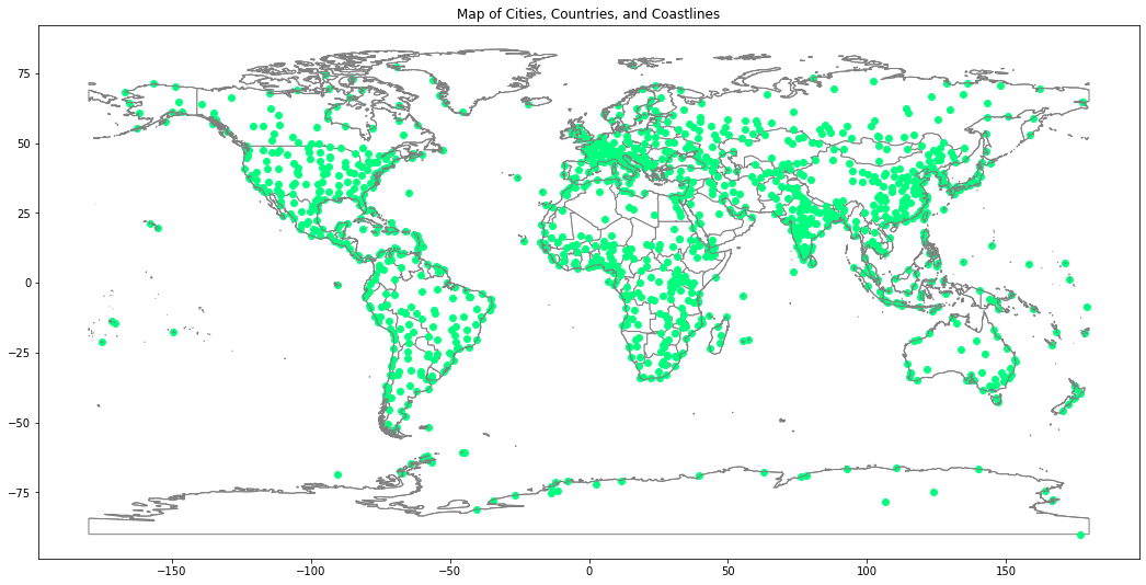
Challenge 2: Create a Global Map
The code below will download one additional file for you that contains global country boundaries. Your goal is to create a map that contains 3 layers:
- the cities or populated places layer that you opened above
- the coastlines layer that you opened above and
- the countries layer that you will open using the code below
To create a map with the three layers, you can:
- Copy the code below that downloads the countries layer.
- Next, use Geopandas
read_file()to open the countries layer as aGeoDataFrame. - Create a map of all three layers - in the same figure using the same
ax=. The countries should be the bottom layer, and the cities and lines should be on top of that layer.
country_data_url = "https://www.naturalearthdata.com/http//www.naturalearthdata.com/download/50m/cultural/ne_50m_admin_0_countries.zip"
et.data.get_data(url=country_data_url)

# Create a path to the countries shapefile
countries_path = os.path.join("data", "earthpy-downloads",
                              "ne_50m_admin_0_countries",
                              "ne_50m_admin_0_countries.shp")
Challenge BONUS: Customize your Map
If you have time, customize your map as follows:
- Adjust the linewidth of lines with
linewidth=4 - Adjust the edge color of polygons using:
edgecolor="grey" - Adjust the color of your objects (the line color, or point color) using:
color='springgreen'.
Finally, add a title to your map using
ax1.set(title="my title here")
Downloading from https://www.naturalearthdata.com/http//www.naturalearthdata.com/download/50m/cultural/ne_50m_admin_0_countries.zip
Extracted output to /root/earth-analytics/data/earthpy-downloads/ne_50m_admin_0_countries
Data Tip: There are many options to customize plots in Python. Below are a few lessons that cover some of this information!
Spatial Data Attributes
Each object in a shapefile has one or more attributes associated with it. Shapefile attributes are similar to fields or columns in a spreadsheet. Each row in the spreadsheet has a set of columns associated with it that describe the row element. In the case of a shapefile, each row represents a spatial object - for example, a road, represented as a line in a line shapefile, will have one “row” of attributes associated with it.
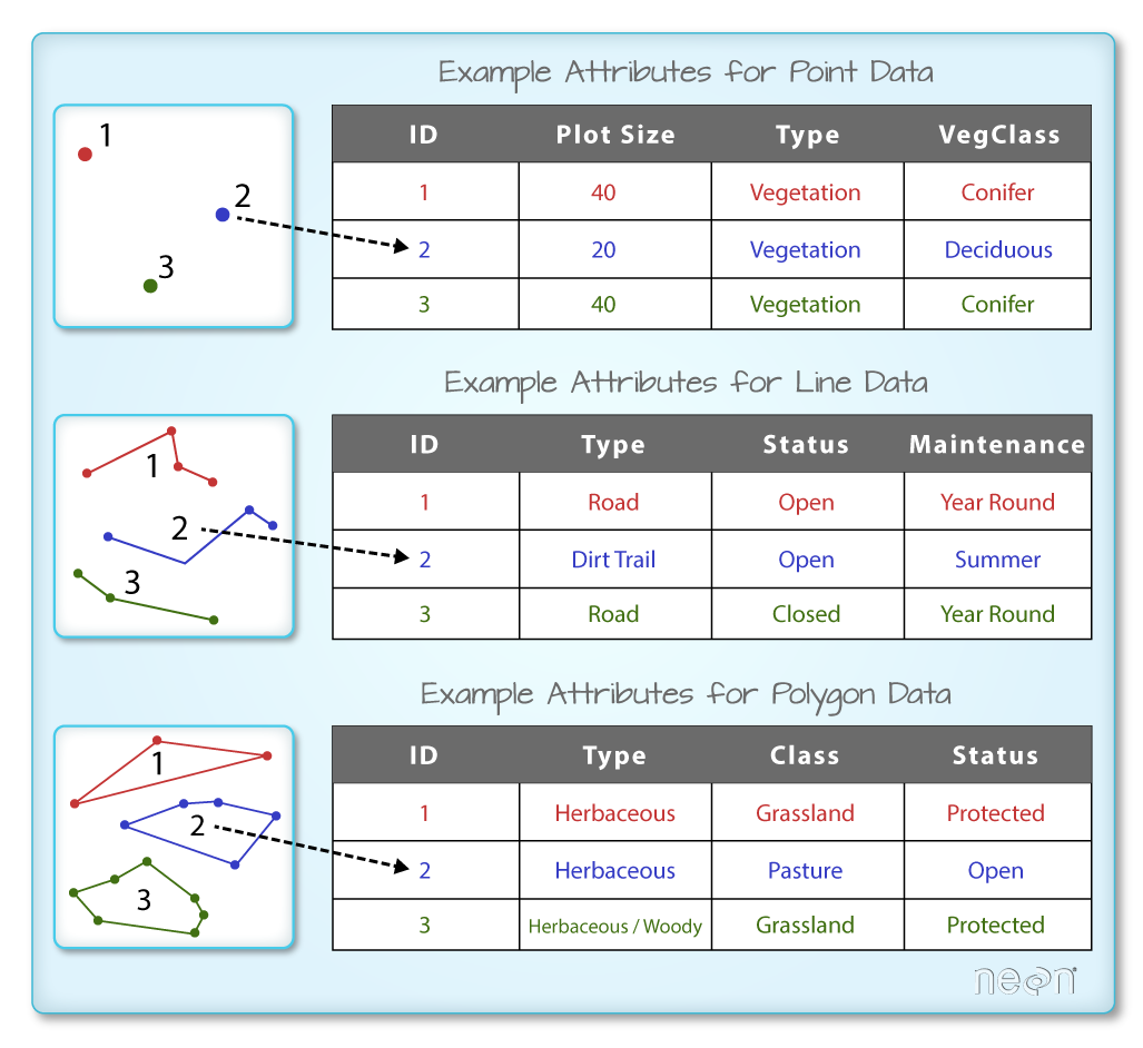
The attributes for a shapefile imported into a GeoDataFrame can be viewed in the GeoDataFrame itself.
# View first 5 rows of GeoDataFrame
cities.head()
| scalerank | natscale | labelrank | featurecla | name | namepar | namealt | diffascii | nameascii | adm0cap | ... | rank_max | rank_min | geonameid | meganame | ls_name | ls_match | checkme | min_zoom | ne_id | geometry | |
|---|---|---|---|---|---|---|---|---|---|---|---|---|---|---|---|---|---|---|---|---|---|
| 0 | 10 | 1 | 5 | Admin-1 region capital | Bombo | None | None | 0 | Bombo | 0.0 | ... | 8 | 7 | 0.0 | None | None | 0 | 0 | 7.0 | 1159113923 | POINT (32.53330 0.58330) |
| 1 | 10 | 1 | 5 | Admin-1 region capital | Fort Portal | None | None | 0 | Fort Portal | 0.0 | ... | 7 | 7 | 233476.0 | None | None | 0 | 0 | 7.0 | 1159113959 | POINT (30.27500 0.67100) |
| 2 | 10 | 1 | 3 | Admin-1 region capital | Potenza | None | None | 0 | Potenza | 0.0 | ... | 8 | 8 | 3170027.0 | None | None | 0 | 0 | 7.0 | 1159117259 | POINT (15.79900 40.64200) |
| 3 | 10 | 1 | 3 | Admin-1 region capital | Campobasso | None | None | 0 | Campobasso | 0.0 | ... | 8 | 8 | 3180991.0 | None | None | 0 | 0 | 7.0 | 1159117283 | POINT (14.65600 41.56300) |
| 4 | 10 | 1 | 3 | Admin-1 region capital | Aosta | None | None | 0 | Aosta | 0.0 | ... | 7 | 7 | 3182997.0 | None | None | 0 | 0 | 7.0 | 1159117361 | POINT (7.31500 45.73700) |
5 rows × 39 columns
# View data just in the pop_max column of the cities object
cities.pop_max
0          75000
1          42670
2          69060
3          50762
4          34062
          ...
1244    11748000
1245    18845000
1246     4630000
1247     5183700
1248     7206000
Name: pop_max, Length: 1249, dtype: int64
Data Tip: Vector Metadata
The spatial and attribute data are not the only important aspects of a shapefile. The metadata of a shapefile are also very important. The metadata includes data on the Coordinate Reference System (CRS), the extent, and much more. For more information on what the metadata is, and how to access it, see the full lesson on vector data on the Earth Lab website, here.</div>
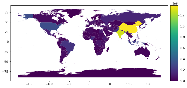
from mpl_toolkits.axes_grid1 import make_axes_locatable

f, ax1 = plt.subplots(figsize=(10, 6))

divider = make_axes_locatable(ax1)
cax = divider.append_axes("right",
                          size="5%",
                          pad=0.1)

countries.plot(column='POP_EST',
               legend=True,
               ax=ax1,
               cax=cax)
plt.show()
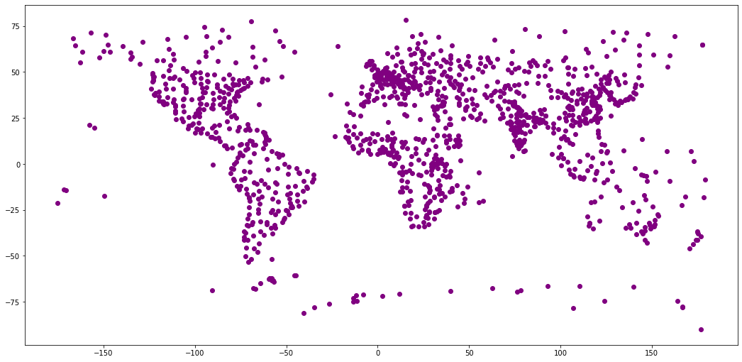
Challenge: Plot Cities Data
Plot the cities object so each point is colored according to the max population value.
HINT: checkout this page on creating maps with Geopandas for more information on customizing maps in Geopandas:
<AxesSubplot:>
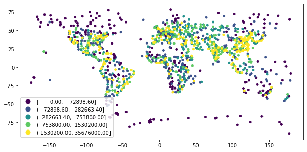
Challenge: Plot Cities Data Using Quantiles – Categorical Plot
You can plot your data according to categorical groups similar to what you might do in a tool like ArcGIS or QGIS. See what happens when you customize your plot code above.
Set the following parameters:
legend=Trueandscheme="quantiles
Optional: Geoprocessing Vector Data Geoprocessing in Python: Clip Data
Sometimes you have spatial data for a larger area than you need to process. For example you may be working on a project for your state or country. But perhaps you have data for the entire globe.
You can clip the data spatially to another boundary to make it smaller. Once the data are clipped, your processing operations will be faster. It will also make creating maps of your study area easier and cleaner.
In the bonus challenge below, you will clip the cities point data to the boundary of a single country. This will make the data smaller and easier to use.
Data Tip: Vector Metadata Check out the spatial data lessons in the intermediate earth-analytics textbook for a more in depth look at clipping data.
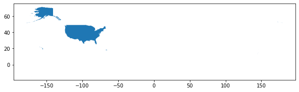
Below you do the following:
- you subset the countries layer to just the boundary of the United State of America
- you then plot the data to look at the newly subsetted data!
- Finally you clip the cities data to only include cities that fall within the boundary of the United States
# Subset the countries data to just a single
united_states_boundary = countries.loc[countries['SOVEREIGNT']
                                       == 'United States of America']

# Notice in the plot below, that only the boundary for the USA is in the new variable
f, ax = plt.subplots(figsize=(10, 6))
united_states_boundary.plot(ax=ax)
plt.show()
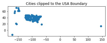
# Clip the cities data to the USA boundary
# Note -- this operation may take some time to run - be patient
cities_in_usa = gpd.clip(cities, united_states_boundary)

# Plot your final clipped data
f, ax = plt.subplots()
cities_in_usa.plot(ax=ax)
ax.set(title="Cities clipped to the USA Boundary")
plt.show()
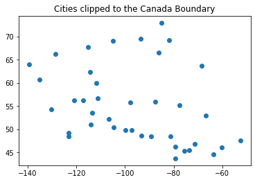
BONUS Challenge: Clip Vector Data in Python
For this bonus challenge, you will clip the cities data that you opened above to the extent of a single country - Canada.
gpd.clip(data_to_clip, boundary_to_clip_to).
Follow the example above to perform your clip operation.
To perform the clip you need the following:
- Create the boundary for Canada by subsetting the countries object
- Clip the cities layer to the Canada boundary layer
- Plot your final cities clipped layer!
When you clip, all of the spatial data outside of the spatial clip boundary (Canada) will not be included in the output dataset.
Share on
Twitter Facebook Google+ LinkedIn
Leave a Comment