Lesson 4. File Formats Exercise
# Importing packages needed to complete this lesson
import os

import pandas as pd
import geopandas as gpd
import matplotlib.pyplot as plt
import earthpy as et
# Creating a home directory
home_dir = os.path.join(et.io.HOME, 'earth-analytics',
                        'data', 'earthpy-downloads')
if not os.path.isdir(home_dir):
    os.makedirs(home_dir)

# Set your working directory
os.chdir(os.path.join(et.io.HOME,
                      'earth-analytics',
                      'data',
                      'earthpy-downloads'))
Challenge 1: Open a Text File
Use the code below to download a .csv file containing data for the climbing formations in the Boulder, Colorado:
et.data.get_data(url="https://opendata.arcgis.com/datasets/175425c25d8849b58feb89483ef02961_1.csv")
Once you have downloaded the data:
- Read the data into Python as a pandas
DataFrame. IMPORTANT: Name your dataframe object boulder_climbing. - View the pandas
DataFrame. Look at the columns in the data. Find theFormationTypecolumn. Notice how it’s categorically split between two different types of formations.
# Download the data that you will use in this lesson
et.data.get_data(
    url="https://opendata.arcgis.com/datasets/175425c25d8849b58feb89483ef02961_1.csv")
Downloading from https://opendata.arcgis.com/datasets/175425c25d8849b58feb89483ef02961_1.csv
'/root/earth-analytics/data/earthpy-downloads/OSMP_Climbing_Formations.csv'
# This code will clean up your file name
# This is a temporary fix for a bug in our earthpy package!
old_name_climb = '"OSMP_Climbing_Formations.csv"'
new_name_climb = 'OSMP_Climbing_Formations.csv'
if not os.path.exists(new_name_climb):
    os.rename(old_name_climb, new_name_climb)
IMPORTANT. When you download the data, you may notice that there are quotes around the file name like this: "OSMP_Climbing_Formations.csv". You will need to call
| X | Y | OBJECTID | ID | FEATURE | ROUTES | HCA | OWNER | SeasonalClosure | AreaAccess | AKA | ClosureActive | PERMITREQ | FormationType | Display | |
|---|---|---|---|---|---|---|---|---|---|---|---|---|---|---|---|
| 0 | -105.294224 | 40.005020 | 1 | 1.0 | Pumpkin Rock | 4.0 | No | OSMP | N | Flagstaff | First Areas | N | No | Boulder | Yes |
| 1 | -105.287861 | 39.975276 | 2 | 2.0 | Veranda | 2.0 | No | OSMP | N | NCAR | NaN | N | No | Wall | Yes |
| 2 | -105.293598 | 39.995411 | 3 | 3.0 | Third Pinnacle | 7.0 | No | OSMP | Y | Gregory Canyon | NaN | N | No | Wall | Yes |
| 3 | -105.294391 | 39.986358 | 4 | 4.0 | The Fin | 1.0 | No | OSMP | Y | Chautauqua | NaN | N | No | Wall | Yes |
| 4 | -105.292811 | 39.995952 | 5 | 6.0 | First Pinnacle | 23.0 | No | OSMP | Y | Gregory Canyon | NaN | N | No | Wall | Yes |
| ... | ... | ... | ... | ... | ... | ... | ... | ... | ... | ... | ... | ... | ... | ... | ... |
| 448 | -105.273410 | 39.985259 | 1177 | NaN | Bro's Spire | NaN | No | OSMP | N | NCAR | NaN | N | No | Boulder | Yes |
| 449 | -105.288583 | 39.978690 | 1178 | NaN | Ridge One (Like Heaven) | NaN | No | OSMP | N | NCAR | NaN | N | No | Boulder | Yes |
| 450 | -105.289838 | 39.978304 | 1179 | NaN | Ridge Two (Satans Slab) | NaN | No | OSMP | Y | NCAR | NaN | N | No | Boulder | Yes |
| 451 | -105.291101 | 39.978087 | 1180 | NaN | Ridge 3 | NaN | No | OSMP | Y | NCAR | NaN | N | No | Boulder | Yes |
| 452 | -105.288788 | 39.965708 | 1181 | NaN | Fiddlehead | NaN | No | OSMP | Y | Cragmoor Rd | NaN | N | No | Wall | Yes |
453 rows × 15 columns
How to Convert x,y Coordinate Data To A GeoDataFrame (or shapefile) - Spatial Data in Tabular Formats
Often you will find that tabular data, stored in a text or spreadsheet format, contains spatial coordinate information that you wish to plot or convert to a shapefile for use in a GIS application. In the challenge below, you will learn how to convert tabular data containing coordinate information into a spatial file.
Challenge 2: Create a Spatial GeoDataframe From a DataFrame
You can create a Geopandas GeoDataFrame from a Pandas DataFrame if there is coordinate data in the DataFrame. In the data that you opened above, there are columns for the X and Y coordinates of each rock formation - with headers named X and Y.
You can convert columns containing x,y coordinate data using the GeoPandas points_from_xy() function as follows:
coordinates = gpd.points_from_xy(column-with-x-data, column-with-y-data.Y)
You can then set the geometry column for the new GeoDataFrame to the x,y data that you extracted from the data frame.
gpd.GeoDataFrame(data=boulder_climbing,
                 geometry=coordinates)
GeoDataFrame. Copy the code below to create a new GeoDataFrame containing the boulder climbing area data in a spatial format that you can plot.
IMPORTANT: be sure to assign the output of the code below to a new variable name called boulder_climbing_gdf.
coordinates = gpd.points_from_xy(boulder_climbing.X, boulder_climbing.Y)
gpd.GeoDataFrame(data=boulder_climbing,
                 geometry=coordinates)
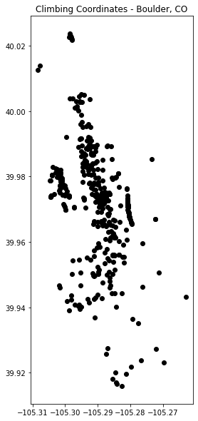
In your code:
- Copy the code above to create a
GeoDataFramefrom theDataFramethat you created above. - Next, plot your data using
.plot()
Data Tip: You can easily export data in a GeoPandas format to a shapefile using object_name_here.to_file("file-name-here.shp"). Following the example above, if you want to export a shapefile called boulder-climbing.shp, your code would look like this: boulder_climbing_gdf.to_file("boulder-climbing.shp").
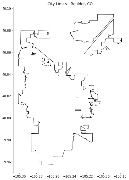
Challenge 3: Create a Base Map
Next, you will create a basemap. Run code below to download another file for boulder. Notice that the data this time are in geojson format rather than a shapefile. Even though the format is different, the data can be worked with using Geopandas in the same way that you would work with a shapefile using read_file().
The data file is:
et.data.get_data(url="https://opendata.arcgis.com/datasets/955e7a0f52474b60a9866950daf10acb_0.geojson")
The code below downloads and cleans up the file name.
# Get the data
et.data.get_data(
    url="https://opendata.arcgis.com/datasets/955e7a0f52474b60a9866950daf10acb_0.geojson")

# This code will clean up your file name
# This is a temporary fix for a bug in our earthpy package!
old_name_city = '"City_Limits.geojson"'
new_name_city = 'City_Limits.geojson'
if not os.path.exists(new_name_city):
    os.rename(old_name_city, new_name_city)
Downloading from https://opendata.arcgis.com/datasets/955e7a0f52474b60a9866950daf10acb_0.geojson
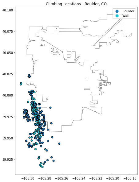
Challenge 4: Plot Two GeoDataFrames Together in the Same Figure
Previously, you learned how to plot multiple shapefiles or spatial layers on the same map using matplotlib.
- Use what you learned in the spatial vector lesson in this chapter to plot the climbing formations points layer on top of the cities boundary that you opened above.
- Use the
edgecolor=and thecolor=parameters to change the colors of the city object. (example: color=”white”, edgecolor=”grey”) - Use
legend=Trueto add a legend to your map. - Set
column='FormationType'to plot your points according tot he type of climbing formation it is (Boulder vs Wall).
HINT: Refer back to the vector lesson if you forget how to create your plot!
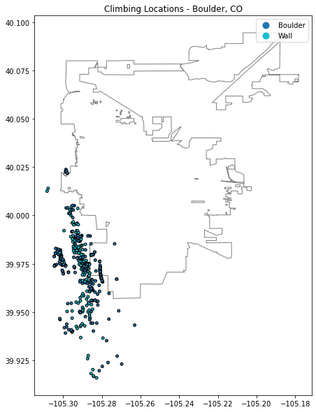
Challenge 5: Customize Your Map
Next, you will customize the map that you created above. Here’s what you need to do to spruce up your map:
- Add a title to your map using
ax.set_title(). - Set the
figsizeof the map to be larger so the data is more clearly shown. Thefigsizeis one of the arguments inplt.subplotsand needs to be set to a tuple of numbers. For example:plt.subplots(figsize=(10, 10). - Turn off the x and y axis data ticks to make the plot look more like a map using:
ax.set_axis_off(). - Customize the colors of the city boundary using the parameters:
color="color-name-here"to change the color of the fill of the polygon. Useedgecolor="color-name-here"to change the outline color of the polygon. HINT: you may want to setcolor="white"for the polygon and make the edgecolor a darker color so you have a clean outline. - Play around with modifying the markers for the points. The marker is the symbol used to represent the x,y location. The default marker is a circle. Modify the
marker=andmarkersize=parameters in theplot()function for the climbing formations in order to make it more legible. Here is a list of marker options in matplotlib: https://matplotlib.org/3.2.1/api/markers_api.html.
Examples of modifying the marker and marker size:
object.plot(marker="*", markersize=5)
OPTIONAL: See what happens when you use the cmap="Greens" argument.
HINT: see this documentation to learn more about color maps in python: https://matplotlib.org/3.2.1/tutorials/colors/colormaps.html
Have fun customizing your map!
OPTIONAL: Interactive Spatial Maps Using Folium
Above you created maps that were static that you could not interact with. You can make interactive maps with Python in Jupyter Notebooks too using the Folium package.
Set your GeoDataFrame name for your climbing formations to the variable specified in the code below, climbing_locations.
import folium

#Define coordinates of where we want to center our map
map_center_coords = [40.015, -105.2705]

#Create the map
my_map = folium.Map(location = map_center_coords, zoom_start = 13)

for lat,long in zip(climbing_locations.geometry.y, climbing_locations.geometry.x):
    folium.Marker(
        location=[lat, long],
    ).add_to(my_map)

my_map
and run it in your code to see what happens!
More reading on how to use Folium here
# In this cell, uncomment the line below.
# This should set your GeoDataFrame to our
# variable name to make the code with folium run

# climbing_locations = boulder_climbing_gdf
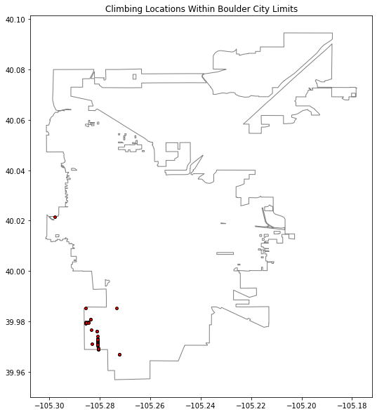
BONUS Challenge: Clip Climbing Formations to the City of Boulder
In the vector notebook, you learned how to clip spatial data. In your code, do the following:
- Clip the climbing formations to the boundary of the city of Boulder.
- Plot the clipped points on top of the city boundary.
If you want, you could create another folium map of the clipped data!
<ipython-input-15-e65987880be3>:5: UserWarning: CRS mismatch between the CRS of left geometries and the CRS of right geometries.
Use `to_crs()` to reproject one of the input geometries to match the CRS of the other.

Left CRS: None
Right CRS: EPSG:4326

  climbing_in_boulder = gpd.clip(boulder_climbing_gdf, city_limits)
Share on
Twitter Facebook Google+ LinkedIn
Leave a Comment