Lesson 3. Run Calculations and Summary Statistics on Pandas Dataframes
Learning Objectives
After completing this page, you will be able to:
- View and sort data in pandas dataframes.
- Run calculations and summary statistics (e.g. mean, minimum, maximum) on columns in pandas dataframes.
Review of Methods and Attributes in Python
Methods in Python
Previous chapters in this textbook have introduced the concept of functions as commands that can take inputs that are used to produce output. For example, you have used many functions, including the print() function to display the results of your code and to write messages about the results.
You have also used functions provided by Python packages such as numpy to run calculations on numpy arrays. For example, you used np.mean() to calculate the average value of specified numpy array. To run these numpy functions, you explicitly provided the name of the variable as an input parameter.
np.mean(arrayname)
In Python, data structures such as pandas dataframes can also provide built-in functions that are referred to as methods. Each data structure has its own set of methods, based on how the data is organized and the types of operations supported by the data structure. A method can be called by adding the .method_name() after the name of the data structure (i.e. object):
object_name.method()
rather than providing the name as an input parameter to a function:
function(object_name)
In this chapter, you will explore some methods (i.e. functions specific to certain objects) that are accessible for pandas dataframes.
Object Attributes in Python
In addition to functions and methods, you have also worked with attributes, which are automatically created characteristics (i.e. metadata) about the data structure or object that you are working with. For example, you used .shape to get the structure (i.e. rows, columns) of a specific numpy array using array.shape. This attribute .shape is automatically generated for a numpy array when it is created.
In this chapter, you will use attributes (i.e. metadata) to get more information about pandas dataframes that is automatically generated when it is created.
Pandas documentation provides a list of all attributes and methods of pandas dataframes.
Import Python Packages and Get Data
Begin by importing the necessary Python packages and then downloading and importing data into pandas dataframes. As you learned previously in this textbook, you can use the earthpy package to download the data files, os to set the working directory, and pandas to import data files into pandas dataframes.
# Import packages
import os

import matplotlib.pyplot as plt
import pandas as pd
import earthpy as et
# URL for .csv with avg monthly precip data
avg_monthly_precip_url = "https://ndownloader.figshare.com/files/12710618"

# Download file
et.data.get_data(url=avg_monthly_precip_url)
'/root/earth-analytics/data/earthpy-downloads/avg-precip-months-seasons.csv'
# Set working directory to earth-analytics
os.chdir(os.path.join(et.io.HOME,
                      "earth-analytics",
                      "data"))
# Import data from .csv file
fname = os.path.join("earthpy-downloads",
                     "avg-precip-months-seasons.csv")

avg_monthly_precip = pd.read_csv(fname)

avg_monthly_precip
| months | precip | seasons | |
|---|---|---|---|
| 0 | Jan | 0.70 | Winter |
| 1 | Feb | 0.75 | Winter |
| 2 | Mar | 1.85 | Spring |
| 3 | Apr | 2.93 | Spring |
| 4 | May | 3.05 | Spring |
| 5 | June | 2.02 | Summer |
| 6 | July | 1.93 | Summer |
| 7 | Aug | 1.62 | Summer |
| 8 | Sept | 1.84 | Fall |
| 9 | Oct | 1.31 | Fall |
| 10 | Nov | 1.39 | Fall |
| 11 | Dec | 0.84 | Winter |
View Contents of Pandas Dataframes
Rather than seeing all of the dataframe at once, you can choose to see the first few rows or the last few rows of a pandas dataframe using the methods .head() or .tail() (e.g. dataframe.tail()).
This capability can be very useful for large datasets which cannot easily be displayed within Jupyter Notebook.
# See first 5 rows
avg_monthly_precip.head()
| months | precip | seasons | |
|---|---|---|---|
| 0 | Jan | 0.70 | Winter |
| 1 | Feb | 0.75 | Winter |
| 2 | Mar | 1.85 | Spring |
| 3 | Apr | 2.93 | Spring |
| 4 | May | 3.05 | Spring |
# See last 5 rows
avg_monthly_precip.tail()
| months | precip | seasons | |
|---|---|---|---|
| 7 | Aug | 1.62 | Summer |
| 8 | Sept | 1.84 | Fall |
| 9 | Oct | 1.31 | Fall |
| 10 | Nov | 1.39 | Fall |
| 11 | Dec | 0.84 | Winter |
Describe Contents of Pandas Dataframes
You can use the method .info() to get details about a pandas dataframe (e.g. dataframe.info()) such as the number of rows and columns and the column names. The output of the .info() method shows you the number of rows (or entries) and the number of columns, as well as the columns names and the types of data they contain (e.g. float64 which is the default decimal type in Python).
# Information about the dataframe
avg_monthly_precip.info()
<class 'pandas.core.frame.DataFrame'>
RangeIndex: 12 entries, 0 to 11
Data columns (total 3 columns):
 #   Column   Non-Null Count  Dtype
---  ------   --------------  -----
 0   months   12 non-null     object
 1   precip   12 non-null     float64
 2   seasons  12 non-null     object
dtypes: float64(1), object(2)
memory usage: 416.0+ bytes
You can also use the attribute .columns to see just the column names in a dataframe, or the attribute .shape to just see the number of rows and columns.
# Get column names
avg_monthly_precip.columns
Index(['months', 'precip', 'seasons'], dtype='object')
# Number of rows and columns
avg_monthly_precip.shape
(12, 3)
Run Summary Statistics on Numeric Values in Pandas Dataframes
Pandas dataframes also provide methods to summarize numeric values contained within the dataframe. For example, you can use the method .describe() to run summary statistics on all of the numeric columns in a pandas dataframe:
dataframe.describe()
such as the count, mean, minimum and maximum values.
The output of .describe() is provided in a nicely formatted dataframe. Note that in the example dataset, the column called precip is the only column with numeric values, so the output of .describe() only includes that column.
# Summary stats of all numeric columns
avg_monthly_precip.describe()
| precip | |
|---|---|
| count | 12.000000 |
| mean | 1.685833 |
| std | 0.764383 |
| min | 0.700000 |
| 25% | 1.192500 |
| 50% | 1.730000 |
| 75% | 1.952500 |
| max | 3.050000 |
Recall that in the lessons on numpy arrays, you ran multiple functions to get the mean, minimum and maximum values of numpy arrays. This fast calculation of summary statistics is one benefit of using pandas dataframes. Note that the .describe() method also provides the standard deviation (i.e. a measure of the amount of variation, or spread, across the data) as well as the quantiles of the pandas dataframes, which tell us how the data are distributed between the minimum and maximum values (e.g. the 25% quantile indicates the cut-off for the lowest 25% values in the data).
You can also run other summary statistics that are not included in describe() such as .median(), .sum(), etc, which provide the output in a pandas series (i.e. a one-dimensional array for pandas).
# Median of all numeric columns
avg_monthly_precip.median()
precip    1.73
dtype: float64
Run Summary Statistics on Individual Columns
You can also run .describe() on individual columns in a pandas dataframe using:
dataframe[["column_name"]].describe()
Note that using the double set of brackets [] around column_name selects the column as a dataframe, and thus, the output is also provided as a dataframe.
# Summary stats on precip column as dataframe
avg_monthly_precip[["precip"]].describe()
| precip | |
|---|---|
| count | 12.000000 |
| mean | 1.685833 |
| std | 0.764383 |
| min | 0.700000 |
| 25% | 1.192500 |
| 50% | 1.730000 |
| 75% | 1.952500 |
| max | 3.050000 |
Using a single set of brackets (e.g. dataframe["column_name"].describe()) selects the column as a pandas series (a one-dimensional array of the column) and thus, the output is also provided as a pandas series.
# Summary stats on precip column as series
avg_monthly_precip["precip"].describe()
count    12.000000
mean      1.685833
std       0.764383
min       0.700000
25%       1.192500
50%       1.730000
75%       1.952500
max       3.050000
Name: precip, dtype: float64
Sort Data Values in Pandas Dataframes
Recall that in the lessons on numpy arrays, you can easily identify the minimum or maximum value, but not the month in which that value occurred. This is because the individual numpy arrays for precip and months were not connected in an easy way that would allow you to determine the month that matches the values.
Using pandas dataframes, you can sort the values with the method .sort_values(), which takes as input:
- the name of the column to sort
- a Boolean value of True or False for the parameter
ascending
dataframe.sort_values(by="column_name", ascending = True)
Using this method, you can sort by the values in the precip column in descending order (ascending = False) to find the maximum value and its corresponding month.
# Sort in descending order for precip
avg_monthly_precip.sort_values(by="precip",
                               ascending=False)
| months | precip | seasons | |
|---|---|---|---|
| 4 | May | 3.05 | Spring |
| 3 | Apr | 2.93 | Spring |
| 5 | June | 2.02 | Summer |
| 6 | July | 1.93 | Summer |
| 2 | Mar | 1.85 | Spring |
| 8 | Sept | 1.84 | Fall |
| 7 | Aug | 1.62 | Summer |
| 10 | Nov | 1.39 | Fall |
| 9 | Oct | 1.31 | Fall |
| 11 | Dec | 0.84 | Winter |
| 1 | Feb | 0.75 | Winter |
| 0 | Jan | 0.70 | Winter |
Run Calculations on Columns Within Pandas Dataframes
You can run mathematical calculations on columns within pandas dataframes using any mathematical calculation and assignment operator such as:
dataframe["column_name"] *= 25.4
which would multiply each value in the column by 25.4.
Using an assignment operator, you can convert the values in the precip column from inches to millimeters (recall that one inch is equal to 25.4 millimeters).
# Convert values from inches to millimeters
avg_monthly_precip["precip"] *= 25.4

avg_monthly_precip
| months | precip | seasons | |
|---|---|---|---|
| 0 | Jan | 17.780 | Winter |
| 1 | Feb | 19.050 | Winter |
| 2 | Mar | 46.990 | Spring |
| 3 | Apr | 74.422 | Spring |
| 4 | May | 77.470 | Spring |
| 5 | June | 51.308 | Summer |
| 6 | July | 49.022 | Summer |
| 7 | Aug | 41.148 | Summer |
| 8 | Sept | 46.736 | Fall |
| 9 | Oct | 33.274 | Fall |
| 10 | Nov | 35.306 | Fall |
| 11 | Dec | 21.336 | Winter |
You can also easily replace or create a new column within a pandas dataframe using mathematical calculations on itself or other columns such as:
dataframe["column_name_2"] = dataframe["column_name_1"] / 25.4
If column_name_2 already exists, then the values are replaced by the calculation (e.g. values in column_name_2 are set to values of column_name_1 divided by 25.4). If column_name_2 does not already exist, then the column is created as the new last column of the dataframe.
The approach below is preferred over directly modifying your existing data!
# Create new column with precip in the original units (inches)
avg_monthly_precip["precip_in"] = avg_monthly_precip["precip"] / 25.4

avg_monthly_precip
| months | precip | seasons | precip_in | |
|---|---|---|---|---|
| 0 | Jan | 17.780 | Winter | 0.70 |
| 1 | Feb | 19.050 | Winter | 0.75 |
| 2 | Mar | 46.990 | Spring | 1.85 |
| 3 | Apr | 74.422 | Spring | 2.93 |
| 4 | May | 77.470 | Spring | 3.05 |
| 5 | June | 51.308 | Summer | 2.02 |
| 6 | July | 49.022 | Summer | 1.93 |
| 7 | Aug | 41.148 | Summer | 1.62 |
| 8 | Sept | 46.736 | Fall | 1.84 |
| 9 | Oct | 33.274 | Fall | 1.31 |
| 10 | Nov | 35.306 | Fall | 1.39 |
| 11 | Dec | 21.336 | Winter | 0.84 |
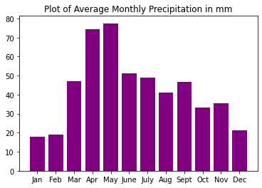
# Plot the data
f, ax = plt.subplots()

ax.bar(x=avg_monthly_precip.months,
       height=avg_monthly_precip.precip,
       color="purple")

ax.set(title="Plot of Average Monthly Precipitation in mm")
plt.show()
Group Values in Pandas Dataframes
Another benefit of pandas dataframes is that you can group data using a shared common value and then summarize the values in another column using those groups. To do this, you can use the following syntax:
dataframe.groupby(['label_column'])[["value_column"]].method()
in which the label_column is the column is used to create the groups and the value_column is the column that will be summarized for each group.
For example, you could group the example dataframe by the seasons and then run the describe() method on precip. This would run .describe() on the precipitation values for each season as a grouped dataset. In this example, the label_column on which you want to group data is seasons and the value_column that you want to summarize is precip.
# Group data by seasons and summarize precip
precip_by_season=avg_monthly_precip.groupby(["seasons"])[["precip"]].describe()
precip_by_season
| precip | ||||||||
|---|---|---|---|---|---|---|---|---|
| count | mean | std | min | 25% | 50% | 75% | max | |
| seasons | ||||||||
| Fall | 3.0 | 38.438667 | 7.257173 | 33.274 | 34.290 | 35.306 | 41.021 | 46.736 |
| Spring | 3.0 | 66.294000 | 16.787075 | 46.990 | 60.706 | 74.422 | 75.946 | 77.470 |
| Summer | 3.0 | 47.159333 | 5.329967 | 41.148 | 45.085 | 49.022 | 50.165 | 51.308 |
| Winter | 3.0 | 19.388667 | 1.802028 | 17.780 | 18.415 | 19.050 | 20.193 | 21.336 |
To plot your grouped data, you will have to adjust the column headings. Above you have what’s called a multiindex dataframe. It has two sets of indexes:
- precip and
- the summary statistics: count, meant, std, etc
precip_by_season.columns
MultiIndex([('precip', 'count'),
            ('precip',  'mean'),
            ('precip',   'std'),
            ('precip',   'min'),
            ('precip',   '25%'),
            ('precip',   '50%'),
            ('precip',   '75%'),
            ('precip',   'max')],
           )
# Drop a level so there is only one index
precip_by_season.columns = precip_by_season.columns.droplevel(0)
precip_by_season
| count | mean | std | min | 25% | 50% | 75% | max | |
|---|---|---|---|---|---|---|---|---|
| seasons | ||||||||
| Fall | 3.0 | 38.438667 | 7.257173 | 33.274 | 34.290 | 35.306 | 41.021 | 46.736 |
| Spring | 3.0 | 66.294000 | 16.787075 | 46.990 | 60.706 | 74.422 | 75.946 | 77.470 |
| Summer | 3.0 | 47.159333 | 5.329967 | 41.148 | 45.085 | 49.022 | 50.165 | 51.308 |
| Winter | 3.0 | 19.388667 | 1.802028 | 17.780 | 18.415 | 19.050 | 20.193 | 21.336 |
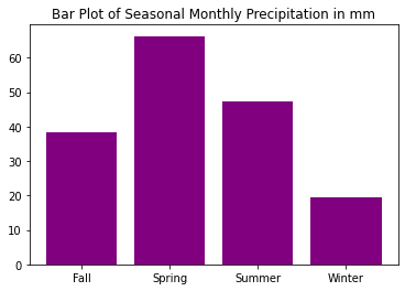
# Plot the data
f, ax = plt.subplots()

ax.bar(precip_by_season.index,
        precip_by_season["mean"],
        color="purple")

ax.set(title="Bar Plot of Seasonal Monthly Precipitation in mm")
plt.show()
In addition to running .describe() using a groupby, you can also run individual statistics such as:
.count()to get the number of rows belonging to a specific group (e.g. season)- other summary statistics such as
.median(),.sum(),.mean(), etc, to calculate these summary statistics by a chosen group
In the example below, a new dataframe is created by running .median() on precip using a groupby on seasons.
# Save median of precip for each season to dataframe
avg_monthly_precip_median = avg_monthly_precip.groupby(
    ["seasons"])[["precip"]].median()

avg_monthly_precip_median
| precip | |
|---|---|
| seasons | |
| Fall | 35.306 |
| Spring | 74.422 |
| Summer | 49.022 |
| Winter | 19.050 |
Note the structure of the new dataframe. Does it look different than other dataframes you have seen?
When you run the .info() on this new dataframe, you will see that the index is now the season names, which means that seasons is no longer a column.
avg_monthly_precip_median.info()
<class 'pandas.core.frame.DataFrame'>
Index: 4 entries, Fall to Winter
Data columns (total 1 columns):
 #   Column  Non-Null Count  Dtype
---  ------  --------------  -----
 0   precip  4 non-null      float64
dtypes: float64(1)
memory usage: 64.0+ bytes
To avoid setting a new index when running summary statistics such as median(), you can add a Boolean value of False for the parameter as_index of groupby() to keep the original index.
# Save to new dataframe with original index
avg_monthly_precip_median = avg_monthly_precip.groupby(
    ["seasons"], as_index=False)[["precip"]].median()

avg_monthly_precip_median
| seasons | precip | |
|---|---|---|
| 0 | Fall | 35.306 |
| 1 | Spring | 74.422 |
| 2 | Summer | 49.022 |
| 3 | Winter | 19.050 |
Reset Index of Pandas Dataframes
You can also easily reset the index of any dataframe back to a range index (i.e. starting at [0]) as needed using the syntax:
dataframe.reset_index(inplace=True)
The inplace=True tells the method reset_index to replace the named dataframe with the reset. Running this syntax on any dataframe will reset the index to a range index (i.e. starting at [0]).
In the example below, the index is reset back to a range index starting at [0], rather than using the season name.
# Save summary stats of precip for each season to dataframe
avg_monthly_precip_stats = avg_monthly_precip.groupby(
    ["seasons"])[["precip"]].describe()

avg_monthly_precip_stats
| precip | ||||||||
|---|---|---|---|---|---|---|---|---|
| count | mean | std | min | 25% | 50% | 75% | max | |
| seasons | ||||||||
| Fall | 3.0 | 38.438667 | 7.257173 | 33.274 | 34.290 | 35.306 | 41.021 | 46.736 |
| Spring | 3.0 | 66.294000 | 16.787075 | 46.990 | 60.706 | 74.422 | 75.946 | 77.470 |
| Summer | 3.0 | 47.159333 | 5.329967 | 41.148 | 45.085 | 49.022 | 50.165 | 51.308 |
| Winter | 3.0 | 19.388667 | 1.802028 | 17.780 | 18.415 | 19.050 | 20.193 | 21.336 |
# Reset index
avg_monthly_precip_stats.reset_index(inplace=True)

avg_monthly_precip_stats
| seasons | precip | ||||||||
|---|---|---|---|---|---|---|---|---|---|
| count | mean | std | min | 25% | 50% | 75% | max | ||
| 0 | Fall | 3.0 | 38.438667 | 7.257173 | 33.274 | 34.290 | 35.306 | 41.021 | 46.736 |
| 1 | Spring | 3.0 | 66.294000 | 16.787075 | 46.990 | 60.706 | 74.422 | 75.946 | 77.470 |
| 2 | Summer | 3.0 | 47.159333 | 5.329967 | 41.148 | 45.085 | 49.022 | 50.165 | 51.308 |
| 3 | Winter | 3.0 | 19.388667 | 1.802028 | 17.780 | 18.415 | 19.050 | 20.193 | 21.336 |
Note in this example that the dataframe is back to a familiar format with a range index starting at [0], but also retains the values calculated with groupby().
You have now learned how to run calculations and summary statistics on columns in pandas dataframes. On the next page, you will learn various ways to select data from pandas dataframes, including indexing and filtering of values.
Share on
Twitter Facebook Google+ LinkedIn
Leave a Comment