Be sure to set your working directory

os.chdir("path-to-you-dir-here/earth-analytics/data")

import os
import numpy as np
import matplotlib.pyplot as plt
import rasterio as rio
from rasterio.plot import show
from rasterio.plot import show_hist
from shapely.geometry import Polygon, mapping
from rasterio.mask import mask
import earthpy as et
import earthpy.spatial as es
import earthpy.plot as ep

from matplotlib.colors import ListedColormap
import matplotlib.colors as colors

# set home directory and download data
et.data.get_data("spatial-vector-lidar")
os.chdir(os.path.join(et.io.HOME, 'earth-analytics'))

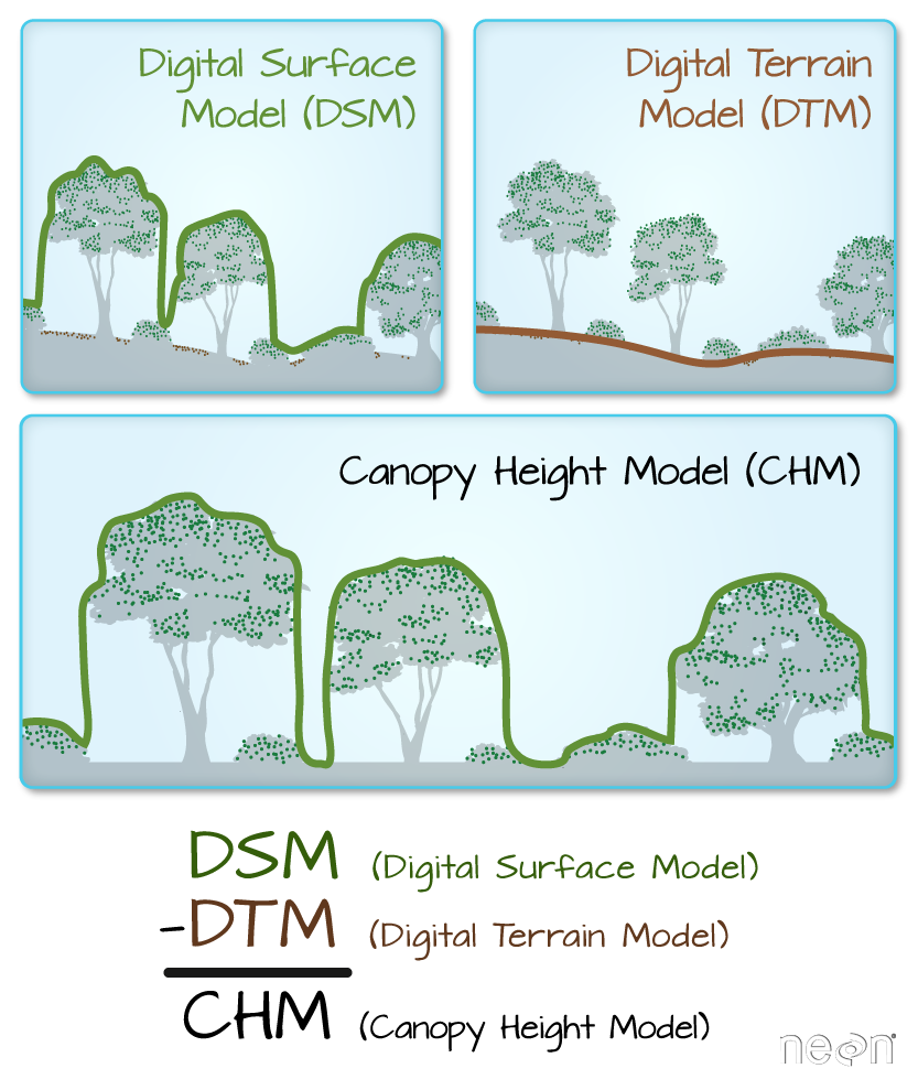
In the previous lesson you learned how to open and plot raster data. In this lesson you’ll learn how to subtract one raster from another. In this example we have a lidar digital surface model and an elevation model. If you subtract elevation from the top of the earth’s surface then you can get tree (and building) heights!

To begin, be sure that you have the digital terrain model data/spatial-vector-lidar/california/neon-soap-site/2013/lidar/SOAP_lidarDTM.tif open already. You used this layer in the previous lesson.

# open the digital terrain model 
sjer_dtm_path = "data/spatial-vector-lidar/california/neon-soap-site/2013/lidar/SOAP_lidarDTM.tif"

with rio.open(sjer_dtm_path) as src:
    lidar_dem_im = src.read(1, masked=True)
    sjer_ext = rio.plot.plotting_extent(src)

Import Digital Surface Model (DSM)

Next, open the digital surface model (DSM). The DSM represents the top of the earth’s surface. Thus, it INCLUDES TREES, BUILDINGS and other objects that sit on the earth.

# open the digital terrain model 
sjer_dsm_path = "data/spatial-vector-lidar/california/neon-soap-site/2013/lidar/SOAP_lidarDSM.tif"

with rio.open(sjer_dsm_path) as src:
    lidar_dsm_im = src.read(1, masked=True)
    dsm_meta = src.profile

lidar_dsm_im

masked_array(
  data=[[1360.4599609375, 1360.3499755859375, 1360.02001953125, ...,
         1020.699951171875, 1020.3599853515625, 1020.7599487304688],
        [1360.4599609375, 1360.27001953125, 1359.8099365234375, ...,
         1006.5399780273438, 1019.0700073242188, 1022.9099731445312],
        [1379.8199462890625, 1362.6500244140625, 1363.22998046875, ...,
         1014.1699829101562, 1016.2699584960938, 1015.2799682617188],
        ...,
        [1318.47998046875, 1321.0499267578125, 1323.72998046875, ...,
         1167.68994140625, 1171.27001953125, 1172.3099365234375],
        [1318.02001953125, 1319.1199951171875, 1322.6300048828125, ...,
         1172.7099609375, 1169.969970703125, 1167.739990234375],
        [1319.419921875, 1319.8399658203125, 1320.3199462890625, ...,
         1182.280029296875, 1179.0, 1171.27001953125]],
  mask=[[False, False, False, ..., False, False, False],
        [False, False, False, ..., False, False, False],
        [False, False, False, ..., False, False, False],
        ...,
        [False, False, False, ..., False, False, False],
        [False, False, False, ..., False, False, False],
        [False, False, False, ..., False, False, False]],
  fill_value=-9999.0,
  dtype=float32)

Canopy Height Model

The canopy height model (CHM) represents the HEIGHT of the trees. This is not an elevation value, rather it’s the height or distance between the ground and the top of the trees (or buildings or whatever object that the lidar system detected and recorded). Some canopy height models also include buildings so you need to look closely are your data to make sure it was properly cleaned before assuming it represents all trees!

Calculate difference between two rasters

There are different ways to calculate a CHM. One easy way is to subtract the DEM from the DSM.

DSM - DEM = CHM

This math gives you the residual value or difference between the top of the earth surface and the ground which should be the heights of the trees (and buildings if the data haven’t been “cleaned”).

Data Tip: Note that this method of subtracting 2 rasters to create a CHM may not give you the most accurate results! There are better ways to create CHM’s using the point clouds themselves. However, in this lesson you learn this method as a means to get more familiar with the CHM dataset and to understand how to perform raster calculations in Python.

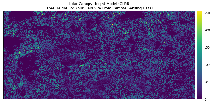
# calculate canopy height model
lidar_chm = lidar_dsm_im - lidar_dem_im

ep.plot_bands(lidar_chm,
              cmap='viridis',
              title="Lidar Canopy Height Model (CHM)\n Tree Height For Your Field Site From Remote Sensing Data!")
plt.show()

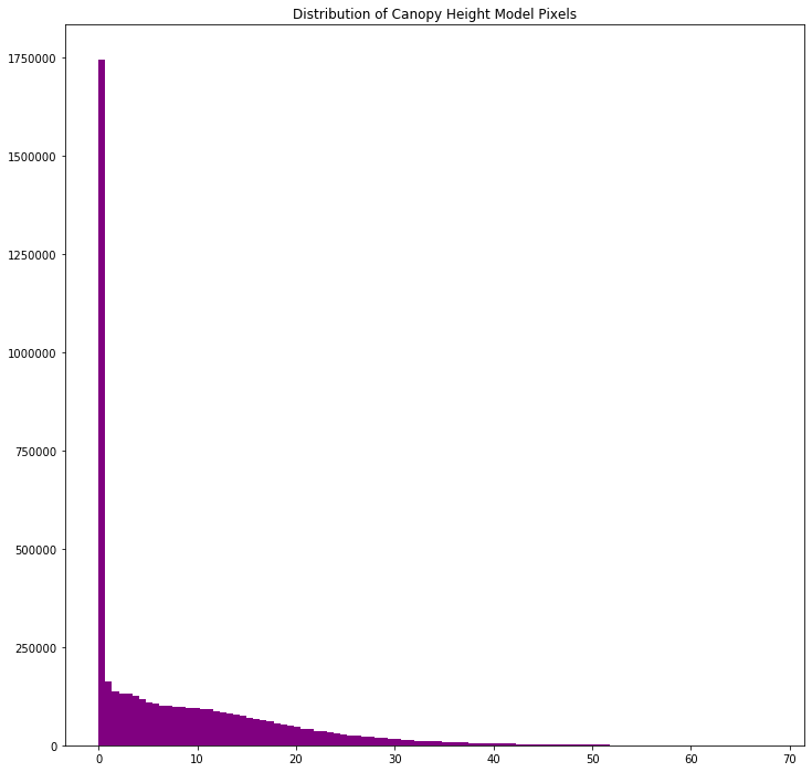
# view histogram of the data
ep.hist(lidar_chm,
        bins=100,
        title="Distribution of Canopy Height Model Pixels")
plt.show()

Take a close look at the output CHM. Do you think that the data just represents trees? Or do you see anything that may suggest that there are other types of objects represented in the data?

Exploring your CHM

Let’s explore your data a bit more to better understand the range of tree (and building) heights that you have in your CHM.

print('CHM minimum value: ', lidar_chm.min())
print('CHM max value: ', lidar_chm.max())

CHM minimum value:  0.0
CHM max value:  68.119995

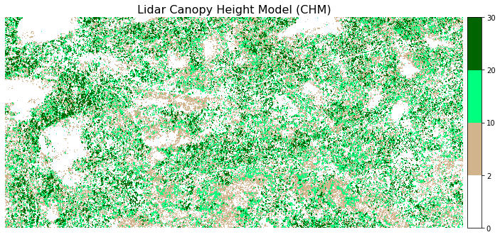
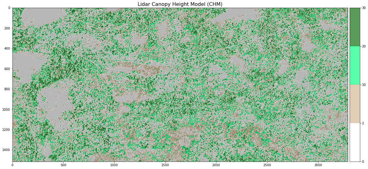
Plots Using Breaks

Sometimes a gradient of colors is useful to represent a continuous variable. But other times, it’s useful to apply colors to particular ranges of values in a raster. These ranges may be statistically generated or simply visually.

Create breaks in your CHM plot.

# Define the colors you want
cmap = ListedColormap(["white", "tan", "springgreen", "darkgreen"])

# Define a normalization from values -> colors
norm = colors.BoundaryNorm([0, 2, 10, 20, 30], 5)

fig, ax = plt.subplots(figsize=(12, 8))
chm_plot = ax.imshow(lidar_chm, 
                     cmap=cmap, 
                     norm=norm)
ax.set_title("Lidar Canopy Height Model (CHM)", fontsize=16)
ep.colorbar(chm_plot)
ax.set_axis_off()
plt.show()

Create a HIllshade and Plot Your Canopy Height Model

# create hillshade using hillshade function in earthpy
chm_hill = es.hillshade(lidar_chm, 315, 45)

# plot the data
fig, ax = plt.subplots(figsize=(20, 20))
ax.imshow(chm_hill, cmap='Greys')
chm_plot = ax.imshow(lidar_chm, 
                     cmap=cmap, 
                     norm=norm, alpha = .65)

ep.colorbar(chm_plot)
ax.set_title("Lidar Canopy Height Model (CHM)", fontsize=16);

O Export a Raster in Python with Rasterio

The last step is option. If you want to share your newly created CHM with a colleague, you may need to export it as a geotiff file.

You can export a raster file in python using the rasterio write() function. Let’s export the canopy height model that you just created to your data folder. You will create a new directory called “outputs” within the week 3 directory. This structure allows you to keep things organized, separating your outputs from the data you downloaded.

NOTE: you can use the code below to check for and create an outputs directory. OR, you can create the directory yourself using the finder (MAC) or windows explorer.

if os.path.exists('data/spatial-vector-lidar/spatial/outputs'):
    print('The directory exists!')
else:
    os.makedirs('data/spatial-vector-lidar/spatial/outputs')

# export chm as a new geotiff to use or share with colleagues
with rio.open('data/spatial-vector-lidar/spatial/outputs/lidar_chm.tiff', 'w', **dsm_meta) as ff:
    ff.write(lidar_chm,1)