Lesson 5. How to Reproject Vector Data in Python Using Geopandas - GIS in Python Spatial data open source python Workshop
Learning Objectives
After completing this tutorial, you will be able to:
- Reproject a vector dataset to another
CRSinPython - Identify the
CRSof a spatial dataset inPython
What You Need
You will need a computer with internet access to complete this lesson and the spatial-vector-lidar data subset created for the course.
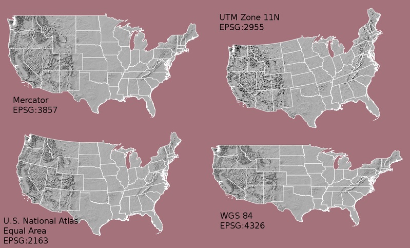
Data in Different Coordinate Reference Systems
Often when data do not line up properly, it is because they are in different coordinate reference systems (CRS). In this lesson you will learn how to reproject data from one CRS to another - so that the data line up properly.
You will use the geopandas, numpy and matplotlib libraries in this tutorial.
Working With Spatial Data From Different Sources
You often need to gather spatial datasets for from different sources and/or data that cover different spatial extents. Spatial data from different sources and that cover different extents are often in different Coordinate Reference Systems (CRS).
Some reasons for data being in different CRSs include:
- The data are stored in a particular CRS convention used by the data provider which might be a federal agency, or a state planning office.
- The data are stored in a particular CRS that is customized to a region. For instance, many states prefer to use a State Plane projection customized for that state.
In this lesson, you will reproject vector data to create a map of the roads near the NEON San Joaquin Experimental Range (SJER) site in Madera County, California.
Import Packages and Data
To get started, import the packages you will need for this lesson into Python and set the current working directory.
# import necessary packages to work with spatial data in Python
import os
import numpy as np
import geopandas as gpd
import matplotlib.pyplot as plt
import earthpy as et

# set home directory and download data
et.data.get_data("spatial-vector-lidar")
os.chdir(os.path.join(et.io.HOME, 'earth-analytics'))
Import the vector data for the Madera County roads and for the boundary of the NEON SJER site.
# import the road data
madera_roads = gpd.read_file("data/spatial-vector-lidar/california/madera-county-roads/tl_2013_06039_roads.shp")

# import the boundary of SJER
# aoi stands for area of interest
sjer_aoi = gpd.read_file("data/spatial-vector-lidar/california/neon-sjer-site/vector_data/SJER_crop.shp")
Identify the CRS
View the CRS of each layer using .crs attribute of geopandas dataframes (e.g. dataframename.crs).
# view the coordinate reference system of both layers
print(madera_roads.crs)
print(sjer_aoi.crs)
{'init': 'epsg:4269'}
{'init': 'epsg:32611'}
Notice that the EPSG codes do not match.
Look up the EPSG codes for 4269 and 32611. What differences do you notice between these coordinate systems?
Next, plot your data. Does anything look off?
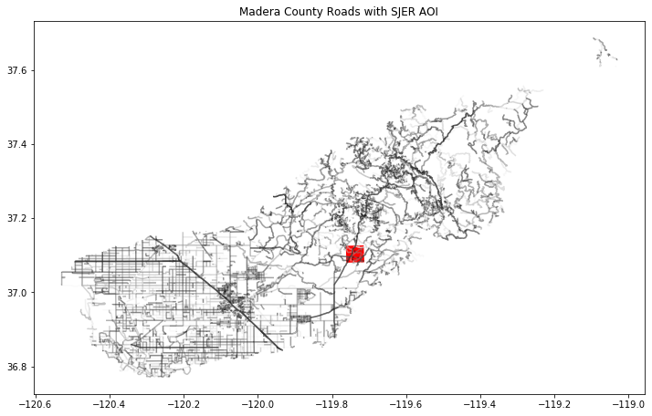
Plot Data
# create the plot
fig, ax = plt.subplots(figsize=(12, 8))
# add roads to the plot
madera_roads.plot(cmap='Greys', ax=ax, alpha=.5)
# add the SJER boundary to the plot
sjer_aoi.plot(ax=ax, markersize=10, color='r')
# add a title for the plot
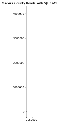
ax.set_title("Madera County Roads with SJER AOI");
Different Data, Same Location, Different Spatial Extents
View the spatial extent of each layer using .total_bounds attribute of geopandas dataframes (e.g. dataframename.total_bounds).
# view the spatial extent of both layers
print(madera_roads.total_bounds)
print(sjer_aoi.total_bounds)
[-120.530241   36.771309 -119.031075   37.686847]
[ 254570.567      4107303.07684455  258867.40933092 4112361.92026107]
Note the difference in the units for each dataset. The spatial extent for the roads is latitude and longitude, while the spatial extent for sjer_aoi is in UTM (meters).
Imagine drawing a box on a grid using these extents. The two extents DO NOT OVERLAP. Yet you know that your data should overlap.
Reproject Vector Data in Geopandas
To plot the data together, they need to be in the same CRS. You can change the CRS, which means you need to reproject the data from one CRS to another CRS using the geopandas method (i.e. function belonging to geopandas objects): to_crs()
The to_crs() method requires two inputs:
- the name of the object that you wish to transform (e.g.
dataframename.to_crs()) - the CRS that you wish to transform that object to (e.g.
dataframename.to_crs(crs-info)) - this can be in the EPSG format or an entire Proj.4 string, which you can find on the Spatial Reference website.
To use the EPSG code, specify the CRS as follows:
'init': 'epsg:4269'
Important: When you reproject data, you are modifying it. Thus, you are introducing some uncertainty into your data. While this is a slightly less important issue when working with vector data (compared to raster), it’s important to consider.
Often you may consider keeping the data that you are doing the analysis on in the correct projection that best relates spatially to the area that you are working in. To get to the point, be sure to use the CRS that best minimizes errors in distance/area/shape, based on your analysis needs.
If you are simply reprojecting to create a base map, then which dataset you reproject matters a lot less because no analysis is involved! However, some people with a keen eye for CRSs may give you a hard time for using the wrong CRS for your study area.
Data Tip: .to_crs() will only work if your original spatial object has a CRS assigned to it AND if that CRS is the correct CRS for that data!
For this lesson, reproject the SJER boundary to match the Madera County roads in EPSG 4269.
Assign a new name to the reprojected data that clearly identifies the CRS. Suggestion: sjer_aoi_wgs84.
# reproject the SJER boundary to match the roads layer using the EPSG code
sjer_aoi_wgs84  = sjer_aoi.to_crs({'init': 'epsg:4269'})
Create a new plot using the reprojected data for the SJER boundary.
# create the plot
fig, ax = plt.subplots(figsize=(12, 8))

# add roads to the plot
madera_roads.plot(cmap='Greys', ax=ax, alpha=.5)

# add the reprojected SJER boundary to the plot
sjer_aoi_wgs84.plot(ax=ax, markersize=10, color='r')

# add a title for the plot
ax.set_title("Madera County Roads with SJER AOI");

Congratulations! You have now reprojected a dataset to be able to map the SJER boundary on top of the Madera County roads layer.
What do you notice about the resultant plot? Can you see where the SJER boundary is within California?
Optional Challenge 1
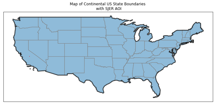
You know what to do! Create a map that includes the following layers:
- United States Boundary:
data/spatial-vector-lidar/usa/usa-boundary-dissolved.shp - State Boundary:
data/spatial-vector-lidar/usa/usa-states-census-2014.shp - SJER AOI:
data/spatial-vector-lidar/california/neon-sjer-site/vector_data/SJER_crop.shp
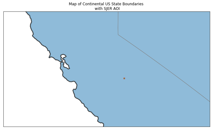
HINT: the SJER boundary is very small relative to the entire United States. Try to zoom in on your map using the following code to set the x and y limits on your plot:
ax.set(xlim=[-125, -116], ylim=[35, 40])
Remember: check the CRS of each dataset!
Optional Challenge 2
The SJER boundary is difficult to see at the full extent of the United States.
You can turn a single polygon into a point using the .centroid() method as follows:
sjer_aoi["geometry"].centroid
Create a plot of the United States with the SJER study site location marked as a POINT marker rather than a polygon. Your map will look like one of the ones below depending upon whether you decide to limit the x and y extents.

<function matplotlib.pyplot.show(*args, **kw)>

Optional Challenge 3
Reproject the original SJER boundary using the full Proj.4 string for EPSG 4269, which you can find on its Spatial Reference webpage and then create the original plot of the Madera County roads and the SJER boundary.
+proj=longlat +ellps=WGS84 +datum=WGS84 +no_defs
Additional Resources - CRS
Share on
Twitter Facebook Google+ LinkedIn
Leave a Comment