Lesson 6. How to Dissolve Polygons Using Geopandas: GIS in Python Spatial data open source python Workshop
Learning Objectives
After completing this tutorial, you will be able to:
- Aggregate the geometry of spatial data using
dissolvebased on an attribute inPython - Aggregate the quantitative values in your attribute table when you perform a dissolve in
Python
What You Need
You will need a computer with internet access to complete this lesson and the spatial-vector-lidar data subset created for the course.
In this lesson, you will use Python to aggregate (i.e. dissolve) the spatial boundaries of the United States state boundaries using a region name that is an attribute of the dataset. Then, you will aggregate the values in the attribute table, so that the quantitative values in the attribute table will reflect the new spatial boundaries for regions.
Import Packages and Data
To get started, import the packages you will need for this lesson into Python and set the current working directory.
# import necessary packages to work with spatial data in Python
import os
import numpy as np
import geopandas as gpd
import matplotlib.pyplot as plt
import matplotlib.lines as mlines
from matplotlib.colors import ListedColormap
import earthpy as et

# set home directory and download data
et.data.get_data("spatial-vector-lidar")
os.chdir(os.path.join(et.io.HOME, 'earth-analytics'))
# import United States state boundaries
state_boundary_us = gpd.read_file("data/spatial-vector-lidar/usa/usa-states-census-2014.shp")
Dissolve Polygons Based On an Attribute with Geopandas
Dissolving polygons entails combining polygons based upon a unique attribute value and removing the interior geometry.
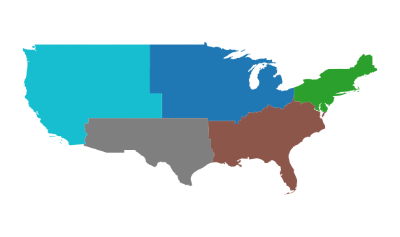
Below you will dissolve the US states polygons by the region that each state is in. When you dissolve, you will create a new set polygons - one for each region in the United States.
To begin, explore your data. Using .geom_type you can see that you have a mix of single and multi polygons in your data. Sometimes multi-polygons can cause problems when processing. It’s always good to check your geometry before you begin to better know what you are working with.
# query the first few records of the geom_type column
state_boundary_us.geom_type.head()
0    MultiPolygon
1         Polygon
2    MultiPolygon
3         Polygon
4         Polygon
dtype: object
Next, select the columns that you with to use for the dissolve and that will be retained.
In this case, we want to retain the columns:
- region
- geometry
# select the columns that you with to use for the dissolve and that will be retained
state_boundary = state_boundary_us[['region', 'geometry']]

# dissolve the state boundary by region
us_regions = state_boundary.dissolve(by='region')

# view the resulting geodataframe
us_regions
| geometry | |
|---|---|
| region | |
| Midwest | (POLYGON Z ((-82.863342 41.693693 0, -82.82571... |
| Northeast | (POLYGON Z ((-76.04621299999999 38.025533 0, -... |
| Southeast | (POLYGON Z ((-81.81169299999999 24.568745 0, -... |
| Southwest | POLYGON Z ((-94.48587499999999 33.637867 0, -9... |
| West | (POLYGON Z ((-118.594033 33.035951 0, -118.540... |
And finally, plot the data. Note that when you dissolve, the column used to perform the dissolve becomes an index for the resultant geodataframe. Thus, you will have to use the reset_index() method when you plot, to access the region column.
If you do not reset the index, the following will return and error, as region is no longer a column, it is an index!
us_regions.plot(column = 'region', ax=ax)
You can use us_regions.reset_index().plot(column = 'region', ax=ax) to reset the index when you plot the data.
# create the plot
fig, ax = plt.subplots(figsize = (10,6))

# plot the data
us_regions.reset_index().plot(column = 'region', ax=ax)

# Set plot axis to equal ratio
ax.set_axis_off()
plt.axis('equal');
Dissolve and Aggregate Data Attributes
In the example above, you dissolved the state level polygons to a region level. However, you did not aggregate or summarize the attributes associated with each polygon.
Next, you will learn how to aggregate quantitative values in your attribute table when you perform a dissolve. To do this, you will add aggfunc = 'summaryfunction' to your dissolve call.
You can choice a suite of different summary functions including:
- first
- last
- mean
- max
And more. Read more about the dissolve function here.
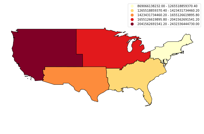
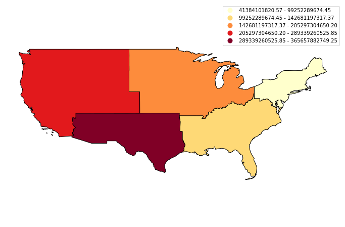
Aggregate the data using the ‘sum’ method on the ALAND and AWATER attributes (total land and water area).
The values for ALAND and AWATER will be added up for all of the states in a region. Those new summed values will be returned in the new dataframe.
# select the columns that you wish to retain in the data
state_boundary = state_boundary_us[['region', 'geometry', 'ALAND', 'AWATER']]

# then summarize the quantative columns by 'sum'
regions_agg = state_boundary.dissolve(by='region', aggfunc = 'sum')

# display the new dataframe
regions_agg
| geometry | ALAND | AWATER | |
|---|---|---|---|
| region | |||
| Midwest | (POLYGON Z ((-82.863342 41.693693 0, -82.82571... | 1943869253244 | 184383393833 |
| Northeast | (POLYGON Z ((-76.04621299999999 38.025533 0, -... | 869066138232 | 108922434345 |
| Southeast | (POLYGON Z ((-81.81169299999999 24.568745 0, -... | 1364632039655 | 103876652998 |
| Southwest | POLYGON Z ((-94.48587499999999 33.637867 0, -9... | 1462631530997 | 24217682268 |
| West | (POLYGON Z ((-118.594033 33.035951 0, -118.540... | 2432336444730 | 57568049509 |
# create the plot
fig, ax = plt.subplots(figsize = (12,8))

# plot the data using a quantile map of the new ALAND values
regions_agg.plot(column = 'ALAND', edgecolor = "black",
                 scheme='quantiles', cmap='YlOrRd', ax=ax,
                 legend = True)


# Set plot axis to equal ratio
ax.set_axis_off()
plt.axis('equal');
Optional Challenge 1
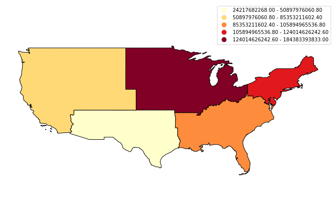
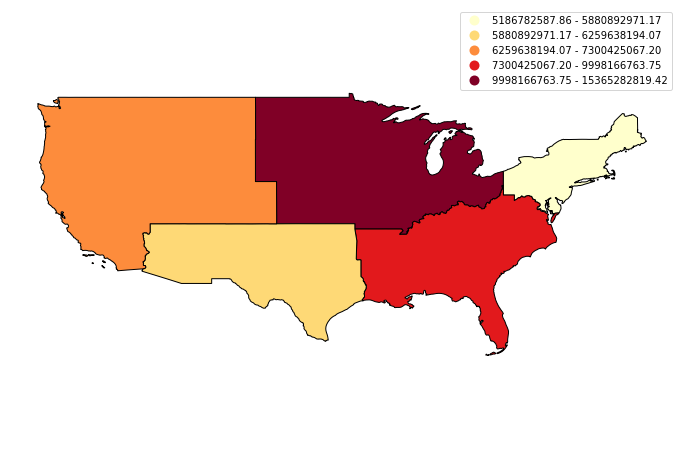
Create a quantile map using the AWATER attribute column.
Optional Challenge 2
Aggregate the data using the ‘mean’ method on the ALAND and AWATER attributes (total land and water area). Then create two maps:
- a map of mean value for ALAND by region and
- a map of mean value for AWATER by region
Share on
Twitter Facebook Google+ LinkedIn
Leave a Comment