Lesson 7. Crop a Spatial Raster Dataset Using a Shapefile in Python Spatial data open source python Workshop
Learning Objectives
After completing this lesson, you will be able to:
- Crop a raster dataset in
Pythonusing a vector extent object derived from a shapefile. - Open a shapefile in
Python.
What You Need
Download spatial-vector-lidar data subset (~172 MB)
You will need a computer with internet access to complete this lesson. If you are following along online and not using our cloud environment:
Get data and software setup instructions here
You will need the Python 3.x Anaconda distribution, git and bash to set things up.
In this lesson, you will learn how to crop a raster dataset in Python.
What Does Crop a Raster Mean?
Cropping (sometimes also referred to as clipping), is when you subset or make a dataset smaller, by removing all data outside of the crop area or spatial extent. In this case you have a large raster - but let’s pretend that you only need to work with a smaller subset of the raster.
You can use the crop_extent function to remove all of the data outside of your study area. This is useful as it:
- Makes the data smaller and
- Makes processing and plotting faster
In general when you can, it’s often a good idea to crop your raster data!
To begin let’s load the libraries that you will need in this lesson.
Load Libraries
Be sure to set your working directory
os.chdir("path-to-you-dir-here/earth-analytics/data")
import os
import numpy as np
import rasterio as rio
from rasterio.plot import show
from rasterio.mask import mask
from shapely.geometry import mapping
import matplotlib.pyplot as plt
import geopandas as gpd
import earthpy as et
import earthpy.plot as ep
import earthpy.spatial as es
import cartopy as cp

# set home directory and download data
et.data.get_data("spatial-vector-lidar")
os.chdir(os.path.join(et.io.HOME, 'earth-analytics'))

# optional - turn off warnings
import warnings
warnings.filterwarnings('ignore')
Open Raster and Vector Layers
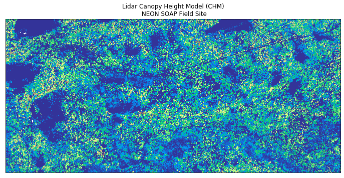
Next, you will use rio.open() to open a raster layer. Open and plot the canopy height model (CHM) that you created in the previous lesson. Or you can use the CHM provided to you in the data directory here:
data/spatial-vector-lidar/california/neon-soap-site/2013/lidar/SOAP_lidarCHM.tif
soap_chm_path = 'data/spatial-vector-lidar/california/neon-soap-site/2013/lidar/SOAP_lidarCHM.tif'
# open the lidar chm
with rio.open(soap_chm_path) as src:
lidar_chm_im = src.read(masked=True)[0]
extent = rio.plot.plotting_extent(src)
soap_profile = src.profile
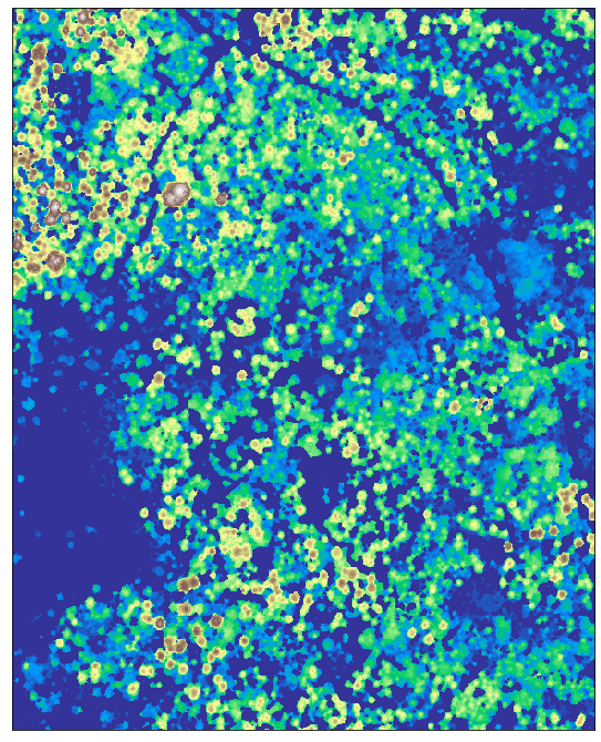
ep.plot_bands(lidar_chm_im,
cmap='terrain',
extent=extent,
title="Lidar Canopy Height Model (CHM)\n NEON SOAP Field Site",
cbar=False);
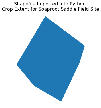
Open Vector Layer
Next, open up a vector layer that contains the crop extent that you want to use to crop your data. To open a shapefile you use the gpd.read_file() function from geopandas.
# open crop extent
crop_extent_soap = gpd.read_file('data/spatial-vector-lidar/california/neon-soap-site/vector_data/SOAP_crop2.shp')
Next, explore the coordinate reference system (CRS) of both of your datasets. Remember that in order to perform any analysis with these two datasets together, they will need to be in the same CRS.
print('crop extent crs: ', crop_extent_soap.crs)
print('lidar crs: ', soap_profile['crs'])
crop extent crs:  {'init': 'epsg:32611'}
lidar crs:  EPSG:32611
# plot the data
fig, ax = plt.subplots(figsize = (6, 6))
crop_extent_soap.plot(ax=ax)
ax.set_title("Shapefile Imported into Python \nCrop Extent for Soaproot Saddle Field Site",
             fontsize = 16)
ax.set_axis_off();
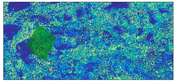
Now that you have imported the shapefile. Plot the two layers together to ensure the overlap each other. If the shapefile does not overlap the raster, then you can not use it to crop!
fig, ax = plt.subplots(figsize=(10, 10))
ep.plot_bands(lidar_chm_im,
              cmap='terrain',
              extent=extent,
              ax=ax,
              cbar=False)
crop_extent_soap.plot(ax=ax, alpha=.6, color='g');
To crop the data,use the crop_image function in earthpy.spatial.
with rio.open(soap_chm_path) as src:
    lidar_chm_crop, soap_lidar_meta = es.crop_image(src, crop_extent_soap)
# Update the metadata to have the new shape (x and y and affine information)
soap_lidar_meta.update({"driver": "GTiff",
                 "height": lidar_chm_crop.shape[0],
                 "width": lidar_chm_crop.shape[1],
                 "transform": soap_lidar_meta["transform"]})

# generate an extent for the newly cropped object for plotting
cr_ext = rio.transform.array_bounds(soap_lidar_meta['height'],
                                            soap_lidar_meta['width'],
                                            soap_lidar_meta['transform'])

bound_order = [0,2,1,3]
cr_extent = [cr_ext[b] for b in bound_order]
cr_extent, crop_extent_soap.total_bounds
([297349.0, 298062.0, 4101114.0, 4101115.0],
 array([ 297349.82145413, 4100402.84616318,  297923.2856659 ,
        4101114.9500745 ]))
# mask the nodata and plot the newly cropped raster layer
lidar_chm_crop_ma = np.ma.masked_equal(lidar_chm_crop[0], -9999.0)
ep.plot_bands(lidar_chm_crop_ma, cmap='terrain', cbar=False);
# Save to disk so you can use the file later.
path_out = "data/spatial-vector-lidar/outputs/soap_lidar_chm_crop.tif"
with rio.open(path_out, 'w', **soap_lidar_meta) as ff:
    ff.write(lidar_chm_crop[0], 1)
Optional Challenge: Crop the SJER Lidar Data
Above your cropped the data for the SOaproot Saddle fieldsite. Crop the data using the same approach for the sjer field site located in this folder: data/spatial-vector-lidar/california/neon-sjer-site.
Share on
Twitter Facebook Google+ LinkedIn
Leave a Comment