Lesson 6. Useful Jupyter Notebook Shortcuts
Learning Objectives
- List useful keyboard shortcuts in
Jupyter Notebook. - Be able to access the list of keyborad shortcuts in
Jupyter Notebook.
List of Useful Jupyter Notebook Shortcuts
Menu Tools vs. Keyboard Shortcuts
As you have seen in this chapter, you can manipulate your Jupyter Notebook using the drop-down tools from the menu, with keyboard shortcuts, or using both.
The table below lists common tasks in Jupyter Notebook and how to do them using keyboard shortcuts or the menu tool.
| Function | Keyboard Shortcut | Menu Tools |
|---|---|---|
| Save notebook | Esc + s | File → Save and Checkpoint |
| Create new cell | Esc + a (above), Esc + b (below) | Insert→ cell above Insert → cell below |
| Run Cell | Ctrl + enter | Cell → Run Cell |
| Copy Cell | c | Copy Key |
| Paste Cell | v | Paste Key |
| Interrupt Kernel | Esc + i i | Kernel → Interrupt |
| Restart Kernel | Esc + 0 0 | Kernel → Restart |
| Find and replace on your code but not the outputs | Esc + f | N/A |
| merge multiple cells | Shift + M | N/A |
| When placed before a function Information about a function from its documentation | ? | N/A |
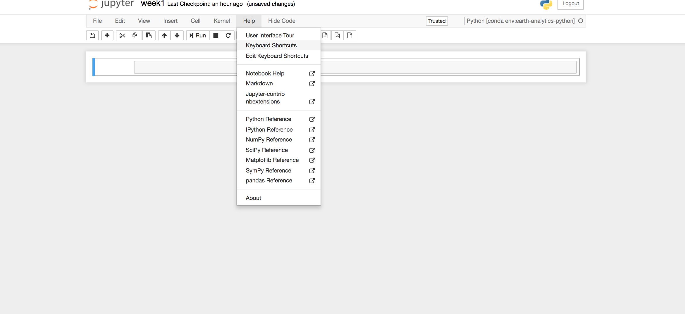
For a full list of keyboard shortcuts, click the help button, then the keyboard shortcuts button.
Additional Resources
Practice Your Jupyter Notebook Skills
Test your Jupyter Notebook skills to:
-
Launch
Jupyter Notebookfrom yourearth-analyticsdirectory. -
Create a new
Jupyter Notebookfile calledjupyter-notebook-interface.ipynb. -
Add a Code cell and copy/paste the following
Pythoncode to determine which day had the most precipitation (i.e. the day of the greatest flooding) during the Fall 2013 flood in Boulder, CO, U.S.A.
# Import necessary packages
import matplotlib.pyplot as plt
import pandas as pd

# Create data
boulder_precip = pd.DataFrame(columns=["date", "precip"],
                              data=[
                                  ["2013-09-09", 0.1], ["2013-09-10", 1.0],
                                  ["2013-09-11", 2.3], ["2013-09-12", 9.8], ["2013-09-13", 1.9],
                                  ["2013-09-14", 0.01], ["2013-09-15", 1.4], ["2013-09-16", 0.4]])
# Create plot
fig, ax = plt.subplots()
ax.bar(boulder_precip['date'].values, boulder_precip['precip'].values)
ax.set(title="Daily Precipitation (inches)\nBoulder, Colorado 2013",
       xlabel="Date", ylabel="Precipitation (Inches)")
plt.setp(ax.get_xticklabels(), rotation=45);
- Run the
Pythoncell.
You have now experienced the benefits of using Jupyter Notebook for open reproducible science!
Without writing your own code, you were able to easily replicate this analysis because this code block can be shared with and run by anyone using Python in Jupyter Notebook.
- Add a Code cell and run each of the following
Pythoncalculations:16 - 424 / 42 * 42 ** 4- What do you notice about the output of
24 / 4compared to the others? - What operation does
**execute?
- What do you notice about the output of
-
Create a new directory called
chap-3in yourearth-analyticsdirectory. -
Create a new directory called
testin yourearth-analyticsdirectory and move it into in the newly created directory calledchap-3. -
Delete the
testdirectory - do you recall how to find thetestdirectory in its new location? -
Rename the
Jupyter Notebookfile that you created in step 2 (e.g.jupyter-notebook-interface.ipynb) using your first initial and last name (e.g.jpalomino-jupyter-notebook-interface.ipynb). -
Create a new folder called
chap-3in yourearth-analyticsdirectory. - Move your renamed
Jupyter Notebookfile (e.g.jpalomino-jupyter-notebook-interface.ipynb) into the newchap-3directory.
Share on
Twitter Facebook Google+ LinkedIn
Leave a Comment