Digital elevation models (DEMs) are data in the format of a 2D array where each cell has a corresponding elevation value. Therefore, it may sometimes prove useful to visualize these elevation models with mechanisms such as contour lines. Fortunately, this is fairly easy to accomplish in Python using packages such as GDAL and Matplotlib.

Objectives

• Read in DEM data
• Visualize data with Matplotlib

Dependencies

• GDAL
• Matplotlib
• numpy
• elevation

from osgeo import gdal
import numpy as np
import matplotlib 
import matplotlib.pyplot as plt
import elevation 

Fetch and read DEM data

The first objective we’ll have to accomplish is acquiring and reading in our data. The data will be downloaded from the NASA SRTM mission via the elevation module’s command line interface.

!eio clip -o Shasta-30m-DEM.tif --bounds -122.6 41.15 -121.9 41.6 

make: Entering directory '/root/.cache/elevation/SRTM1'
make: Nothing to be done for 'download'.
make: Leaving directory '/root/.cache/elevation/SRTM1'
make: Entering directory '/root/.cache/elevation/SRTM1'
make: Nothing to be done for 'all'.
make: Leaving directory '/root/.cache/elevation/SRTM1'
make: Entering directory '/root/.cache/elevation/SRTM1'
cp SRTM1.vrt SRTM1.f7f22bf952f4480f909aba74e2cc9972.vrt
make: Leaving directory '/root/.cache/elevation/SRTM1'
make: Entering directory '/root/.cache/elevation/SRTM1'
gdal_translate -q -co TILED=YES -co COMPRESS=DEFLATE -co ZLEVEL=9 -co PREDICTOR=2 -projwin -122.6 41.6 -121.9 41.15 SRTM1.f7f22bf952f4480f909aba74e2cc9972.vrt /root/earth-analytics-lessons/Shasta-30m-DEM.tif
rm -f SRTM1.f7f22bf952f4480f909aba74e2cc9972.vrt
make: Leaving directory '/root/.cache/elevation/SRTM1'

We can use GDAL in order to open the file and read it in as a 2D array. Additionally, it is important to note that our DEM file has NaN values which will later cause Matplotlib to fail. Therefore, we’ll also mask these values out so that Matplotlib will be unaware of them.

filename = "Shasta-30m-DEM.tif"
gdal_data = gdal.Open(filename)
gdal_band = gdal_data.GetRasterBand(1)
nodataval = gdal_band.GetNoDataValue()

# convert to a numpy array
data_array = gdal_data.ReadAsArray().astype(np.float)
data_array

# replace missing values if necessary
if np.any(data_array == nodataval):
    data_array[data_array == nodataval] = np.nan

Visualize Data with Matplotlib

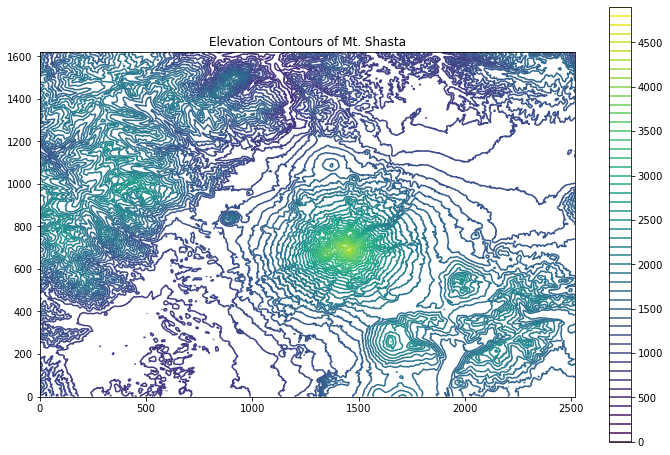
Now that we’ve read our data in, we’re ready to visualize the elevation using contour lines within Matplotlib (Note: We will be re-reading in the data again here due to NaN values).

#Plot out data with Matplotlib's 'contour'
fig = plt.figure(figsize = (12, 8))
ax = fig.add_subplot(111)
plt.contour(data_array, cmap = "viridis", 
            levels = list(range(0, 5000, 100)))
plt.title("Elevation Contours of Mt. Shasta")
cbar = plt.colorbar()
plt.gca().set_aspect('equal', adjustable='box')
plt.show()

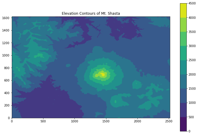
We just used the ‘contour’ module to plot our data. Let’s do it again but with ‘contourf’ to see filled contours.

#Plot our data with Matplotlib's 'contourf'
fig = plt.figure(figsize = (12, 8))
ax = fig.add_subplot(111)
plt.contourf(data_array, cmap = "viridis", 
            levels = list(range(0, 5000, 500)))
plt.title("Elevation Contours of Mt. Shasta")
cbar = plt.colorbar()
plt.gca().set_aspect('equal', adjustable='box')
plt.show()