Computing raster statistics around buffered spatial points Python
One important thing we can do with data in Raster format is calculate statistical values such as mean, standard deviation, variance, etc. around points in the data. By doing so, we’re able to find out attributes about the data and can generalize areas of it as opposed to dealing with every single individual cell.
Objectives
- Read in a GeoTIFF
- Extract data from the raster at buffered point locations
- Compute statistics from these points
Dependencies
- GDAL
- NumPy
- GeoPy
- Matplotlib
- elevation
from __future__ import division
from geopy.geocoders import Nominatim
from osgeo import gdal
import matplotlib.pyplot as plt
import numpy as np
import elevation
Download and read the Data
Our first objective is to read in the data that we want to use. We’ll be working with .tiff image files and reading these in as numpy arrays. By doing so, we’ll be able to essentially “view” our image as a 2D array where each cell corresponds to some value stored in each pixel of the image.
!eio selfcheck
'unzip' not found or not usable.
!eio clip -o Shasta-30m-DEM.tif --bounds -122.6 41.15 -121.9 41.6
make: Entering directory '/root/.cache/elevation/SRTM1'
curl -s -o spool/N41/N41W123.hgt.gz.temp https://s3.amazonaws.com/elevation-tiles-prod/skadi/N41/N41W123.hgt.gz && mv spool/N41/N41W123.hgt.gz.temp spool/N41/N41W123.hgt.gz
gunzip spool/N41/N41W123.hgt.gz 2>/dev/null || touch spool/N41/N41W123.hgt
gdal_translate -q -co TILED=YES -co COMPRESS=DEFLATE -co ZLEVEL=9 -co PREDICTOR=2 spool/N41/N41W123.hgt cache/N41/N41W123.tif 2>/dev/null || touch cache/N41/N41W123.tif
curl -s -o spool/N41/N41W122.hgt.gz.temp https://s3.amazonaws.com/elevation-tiles-prod/skadi/N41/N41W122.hgt.gz && mv spool/N41/N41W122.hgt.gz.temp spool/N41/N41W122.hgt.gz
gunzip spool/N41/N41W122.hgt.gz 2>/dev/null || touch spool/N41/N41W122.hgt
gdal_translate -q -co TILED=YES -co COMPRESS=DEFLATE -co ZLEVEL=9 -co PREDICTOR=2 spool/N41/N41W122.hgt cache/N41/N41W122.tif 2>/dev/null || touch cache/N41/N41W122.tif
rm spool/N41/N41W123.hgt spool/N41/N41W122.hgt
make: Leaving directory '/root/.cache/elevation/SRTM1'
make: Entering directory '/root/.cache/elevation/SRTM1'
gdalbuildvrt -q -overwrite SRTM1.vrt cache/N41/N41W123.tif cache/N41/N41W122.tif
make: Leaving directory '/root/.cache/elevation/SRTM1'
make: Entering directory '/root/.cache/elevation/SRTM1'
cp SRTM1.vrt SRTM1.a696d7f97ba14cb8b8f7fda62dc521e5.vrt
make: Leaving directory '/root/.cache/elevation/SRTM1'
make: Entering directory '/root/.cache/elevation/SRTM1'
gdal_translate -q -co TILED=YES -co COMPRESS=DEFLATE -co ZLEVEL=9 -co PREDICTOR=2 -projwin -122.6 41.6 -121.9 41.15 SRTM1.a696d7f97ba14cb8b8f7fda62dc521e5.vrt /root/earth-analytics-lessons/Shasta-30m-DEM.tif
rm -f SRTM1.a696d7f97ba14cb8b8f7fda62dc521e5.vrt
make: Leaving directory '/root/.cache/elevation/SRTM1'
filename = "Shasta-30m-DEM.tif"
gdal_data = gdal.Open(filename)
gdal_band = gdal_data.GetRasterBand(1)
nodataval = gdal_band.GetNoDataValue()
data_array = gdal_data.ReadAsArray().astype(np.float)
data_array
array([[1066., 1064., 1064., ..., 1450., 1451., 1451.],
       [1067., 1065., 1064., ..., 1451., 1452., 1452.],
       [1067., 1065., 1064., ..., 1452., 1452., 1453.],
       ...,
       [1589., 1594., 1592., ..., 1089., 1091., 1093.],
       [1591., 1595., 1592., ..., 1069., 1068., 1070.],
       [1598., 1599., 1596., ..., 1049., 1048., 1051.]])
# replace missing values if necessary
if np.any(data_array == nodataval):
    data_array[data_array == nodataval] = np.nan

#View the data we're using
plt.figure(figsize = (8, 8))
plt.axis("off")
img = plt.imshow(data_array, cmap = "viridis")
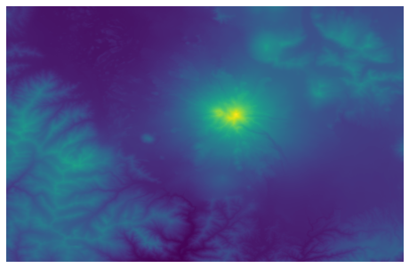
Our goal is to extract information from this raster around a point. To define a spatial location, we need to know what the projection is for our digital elevation model. We can do this with the GetProjection method:
prj = gdal_data.GetProjection()
print(prj)
GEOGCS["WGS 84",DATUM["WGS_1984",SPHEROID["WGS 84",6378137,298.257223563,AUTHORITY["EPSG","7030"]],AUTHORITY["EPSG","6326"]],PRIMEM["Greenwich",0],UNIT["degree",0.0174532925199433,AUTHORITY["EPSG","9122"]],AXIS["Latitude",NORTH],AXIS["Longitude",EAST],AUTHORITY["EPSG","4326"]]
Extracting raster data around point locations
Now that we’ve read in our data, and we know what spatial coordinate system we are in, we’re ready to extract a subset of this data that we want to compute statistics on. In doing so, we’ll be able to get averages and other attributes from an area of our data as opposed to simply looking at individual values from pixels. Let’s extract these points from a circular buffer that we’ll place onto the data.
We’ll first need to define where to center our circle buffer. Let’s do this by using the central lat/lon coordinates for the city of Mt. Shasta, which we’ll get by using the GeoPy module.
# Find coordinates of where we want to center our circle
def get_latlon(city_name):
    geolocator = Nominatim(user_agent="raster-extraction-tutorial")
    latlon = geolocator.geocode(city_name)
    return latlon

coords = get_latlon("Mt. Shasta, CA")
coords
Location(Mount Shasta, Siskiyou County, California, United States of America, (41.4091897, -122.1949533, 0.0))
Next, we need to find the row and column index for our point, which is currently defined as a latitude/longitidue tuple.
#Get row and column in raster based upon coordinates
#This is where we'll center the circle
def get_coords_at_point(rasterfile, pos):
gdata = gdal.Open(rasterfile)
gt = gdata.GetGeoTransform()
data = gdata.ReadAsArray().astype(np.float)
row = int((pos[1] - gt[0])/gt[1])
col = int((pos[0] - gt[3])/gt[5])
return col, row
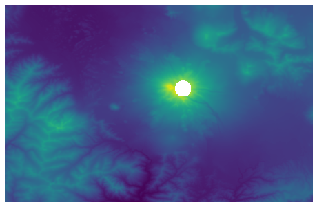
radius = 60 # in units of pixels
row, col = get_coords_at_point(filename, pos = coords[1])
circle = (row, col, radius)
#Extract the points within the circle
def points_in_circle(circle, arr):
    buffer_points = []
    i0, j0, r = circle

    def int_ceiling(x):
        return int(np.ceil(x))

    for i in range(int_ceiling(i0 - r), int_ceiling(i0 + r)):
        ri = np.sqrt(r**2 - (i - i0)**2)

        for j in range(int_ceiling(j0 - ri), int_ceiling(j0 + ri)):
            buffer_points.append(arr[i][j])
            arr[i][j] = np.nan

    return buffer_points

buffer_points = points_in_circle(circle, data_array)
fig = plt.figure(figsize = (8, 8))
ax = fig.add_subplot(111)
plt.axis("off")
img = plt.imshow(data_array, cmap = "viridis")
Compute Statistics
Now that we have all of the values within the buffer/area, we can use NumPy to compute statistics such as mean, standard deviation, and variance on the data.
mean = np.nanmean(buffer_points)
std = np.nanstd(buffer_points)
variance = np.nanvar(buffer_points)

print("Mean: %.2f" % mean)
print("Standard Deviation: %.2f" % std)
print("Variance: %.2f" % variance)
Mean: 3746.62
Standard Deviation: 231.50
Variance: 53592.80
Share on
Twitter Facebook Google+ LinkedIn
Leave a Comment