Get EDDI data over a region of interest and save a GeoTIFF
Maxwell B. Joseph
2019-05-23
Source:vignettes/eddi-roi-tutorial.Rmd
eddi-roi-tutorial.RmdThe eddi R package provides easy access to the Evaporative Demand Drought Index (EDDI) data - an experimental drought monitoring and early warning guidance tool produced by the National Oceanic and Atmospheric Administration. EDDI is available at multiple timescales, from weekly to monthly, providing insight into short-term flash droughts, and long-term droughts. More information on the EDDI product is available on the NOAA EDDI homepage.
This vignette covers a common use case for EDDI: acquiring data over a region of interest defined by a shapefile, masking the EDDI data to that region, and saving GeoTIFF files containing EDDI data for the region of interest.
Defining a region of interest
By default, the eddi package returns data for the continental United States, southern parks of Canada, and northern parts of Mexico. But, you may only be interested in a region of interest, as defined by a shapefile. Here, you will load a shapefile for the state of North Carolina that is distributed by default with the sf package.
library(sf)
#> Linking to GEOS 3.6.2, GDAL 2.2.3, PROJ 4.9.3
library(raster)
#> Loading required package: sp
library(eddi)

roi <- st_read(system.file("shape/nc.shp", package="sf"))
#> Reading layer `nc' from data source `/home/max/R/x86_64-pc-linux-gnu-library/3.6/sf/shape/nc.shp' using driver `ESRI Shapefile'
#> Simple feature collection with 100 features and 14 fields
#> geometry type:  MULTIPOLYGON
#> dimension:      XY
#> bbox:           xmin: -84.32385 ymin: 33.88199 xmax: -75.45698 ymax: 36.58965
#> epsg (SRID):    4267
#> proj4string:    +proj=longlat +datum=NAD27 +no_defs
If you are using a different shapefile, replace system.file("shape/nc.shp", package="sf") with its file path, e.g., st_read("path/to/file.shp").
The roi object contains multiple columns of data, and a geometry column that contains spatial information on the region of interest, which in this case consists of multiple counties.
roi
#> Simple feature collection with 100 features and 14 fields
#> geometry type:  MULTIPOLYGON
#> dimension:      XY
#> bbox:           xmin: -84.32385 ymin: 33.88199 xmax: -75.45698 ymax: 36.58965
#> epsg (SRID):    4267
#> proj4string:    +proj=longlat +datum=NAD27 +no_defs
#> First 10 features:
#>     AREA PERIMETER CNTY_ CNTY_ID        NAME  FIPS FIPSNO CRESS_ID BIR74
#> 1  0.114     1.442  1825    1825        Ashe 37009  37009        5  1091
#> 2  0.061     1.231  1827    1827   Alleghany 37005  37005        3   487
#> 3  0.143     1.630  1828    1828       Surry 37171  37171       86  3188
#> 4  0.070     2.968  1831    1831   Currituck 37053  37053       27   508
#> 5  0.153     2.206  1832    1832 Northampton 37131  37131       66  1421
#> 6  0.097     1.670  1833    1833    Hertford 37091  37091       46  1452
#> 7  0.062     1.547  1834    1834      Camden 37029  37029       15   286
#> 8  0.091     1.284  1835    1835       Gates 37073  37073       37   420
#> 9  0.118     1.421  1836    1836      Warren 37185  37185       93   968
#> 10 0.124     1.428  1837    1837      Stokes 37169  37169       85  1612
#>    SID74 NWBIR74 BIR79 SID79 NWBIR79                       geometry
#> 1      1      10  1364     0      19 MULTIPOLYGON (((-81.47276 3...
#> 2      0      10   542     3      12 MULTIPOLYGON (((-81.23989 3...
#> 3      5     208  3616     6     260 MULTIPOLYGON (((-80.45634 3...
#> 4      1     123   830     2     145 MULTIPOLYGON (((-76.00897 3...
#> 5      9    1066  1606     3    1197 MULTIPOLYGON (((-77.21767 3...
#> 6      7     954  1838     5    1237 MULTIPOLYGON (((-76.74506 3...
#> 7      0     115   350     2     139 MULTIPOLYGON (((-76.00897 3...
#> 8      0     254   594     2     371 MULTIPOLYGON (((-76.56251 3...
#> 9      4     748  1190     2     844 MULTIPOLYGON (((-78.30876 3...
#> 10     1     160  2038     5     176 MULTIPOLYGON (((-80.02567 3...
Because you don’t necessarily care about each county, but rather you want the entire state (including all counties) you can use a spatial union to join data from all counties:
roi <- st_union(roi)
roi
#> Geometry set for 1 feature
#> geometry type:  MULTIPOLYGON
#> dimension:      XY
#> bbox:           xmin: -84.32385 ymin: 33.88199 xmax: -75.45698 ymax: 36.58965
#> epsg (SRID):    4267
#> proj4string:    +proj=longlat +datum=NAD27 +no_defs
#> MULTIPOLYGON (((-76.54427 34.58783, -76.55515 3...
Acquiring EDDI data
To acquire EDDI data, you can use the get_eddi() function. You will fetch the 1 week timescale data for July, 2018:
The eddi_raster object is a RasterStack with one layer, and you can see information on the spatial extent, resolution, and coordinate reference system by printing the object:
eddi_raster
#> class      : RasterStack
#> dimensions : 224, 464, 103936, 1  (nrow, ncol, ncell, nlayers)
#> resolution : 0.125, 0.125  (x, y)
#> extent     : -125, -67, 25, 53  (xmin, xmax, ymin, ymax)
#> crs        : +init=epsg:4326 +proj=longlat +datum=WGS84 +no_defs +ellps=WGS84 +towgs84=0,0,0
#> names      : EDDI_ETrs_01wk_20180701
Plot the data with a custom color palette to see what the data look like:
color_pal <- colorRampPalette(c("blue", "lightblue", "white", "pink", "red"))
plot(eddi_raster, col = color_pal(255))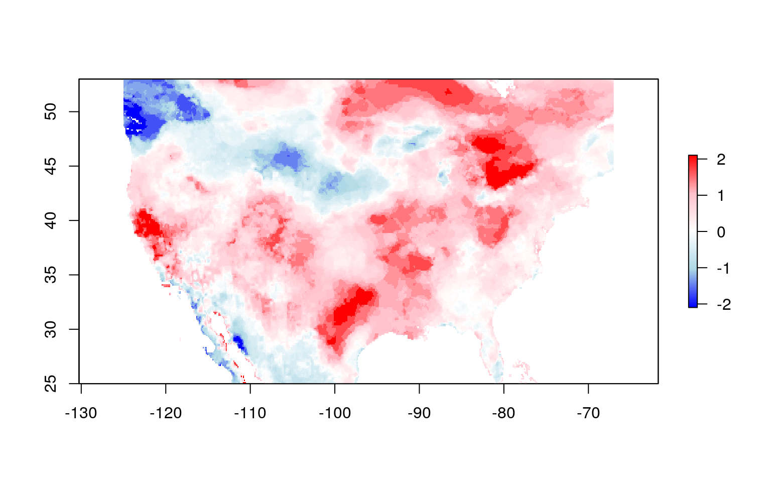
Masking to the region of interest
Now you want to subset or mask the EDDI data to the region of interest. First, you need to ensure that the raster data and the polygon for the region of interest have the same coordinate reference system.
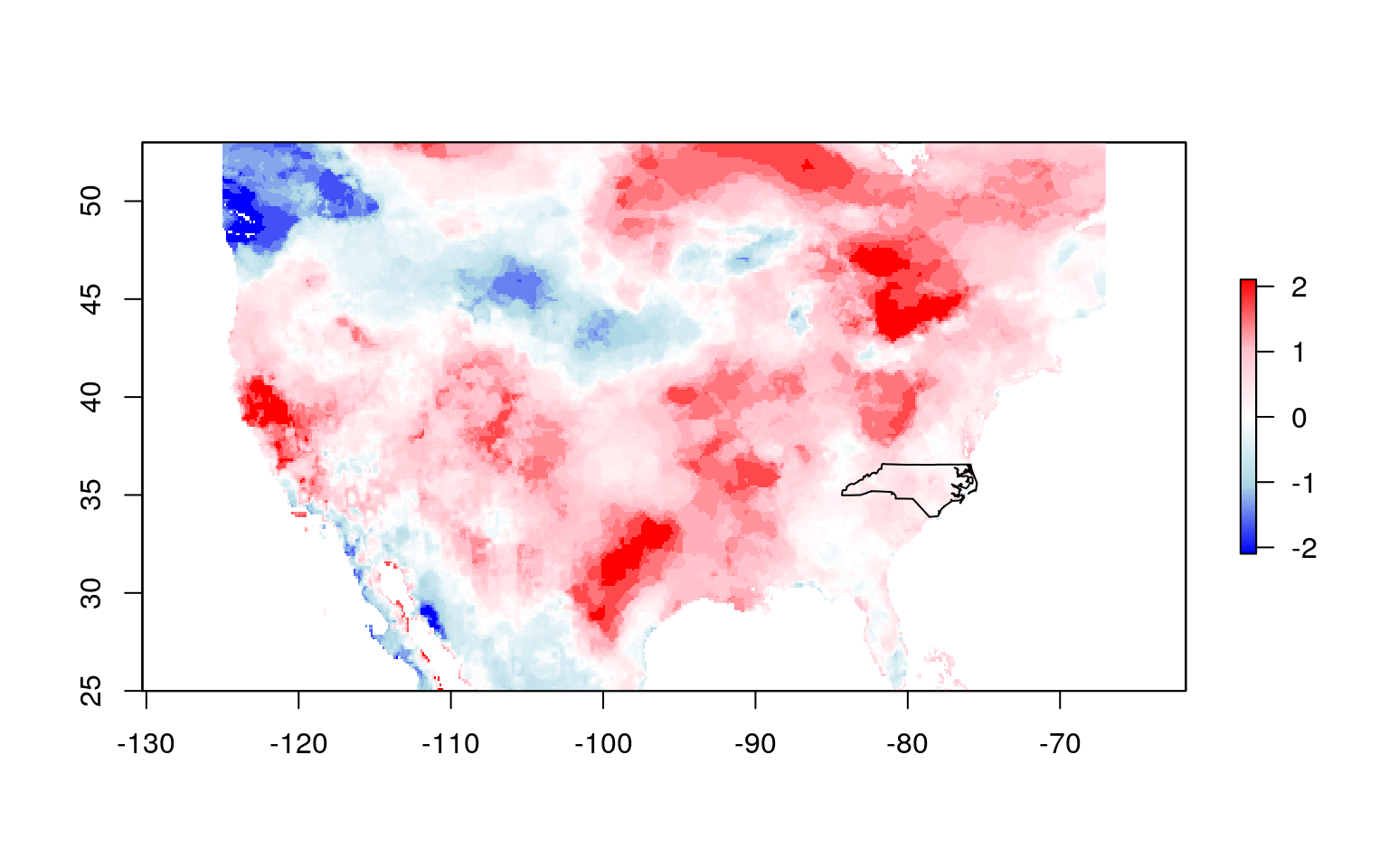
Now, graphically verify that they align as expected:
Now, you can crop the EDDI data to match extents with the region of interest, then mask the raster set all values outside of the region of interest to NA. Because the raster package requires sp objects, rather than sf objects, you will coerce our roi to a sp object first.
roi_sp <- as(roi_reprojected, 'Spatial')
cropped_eddi <- crop(eddi_raster, roi_sp)
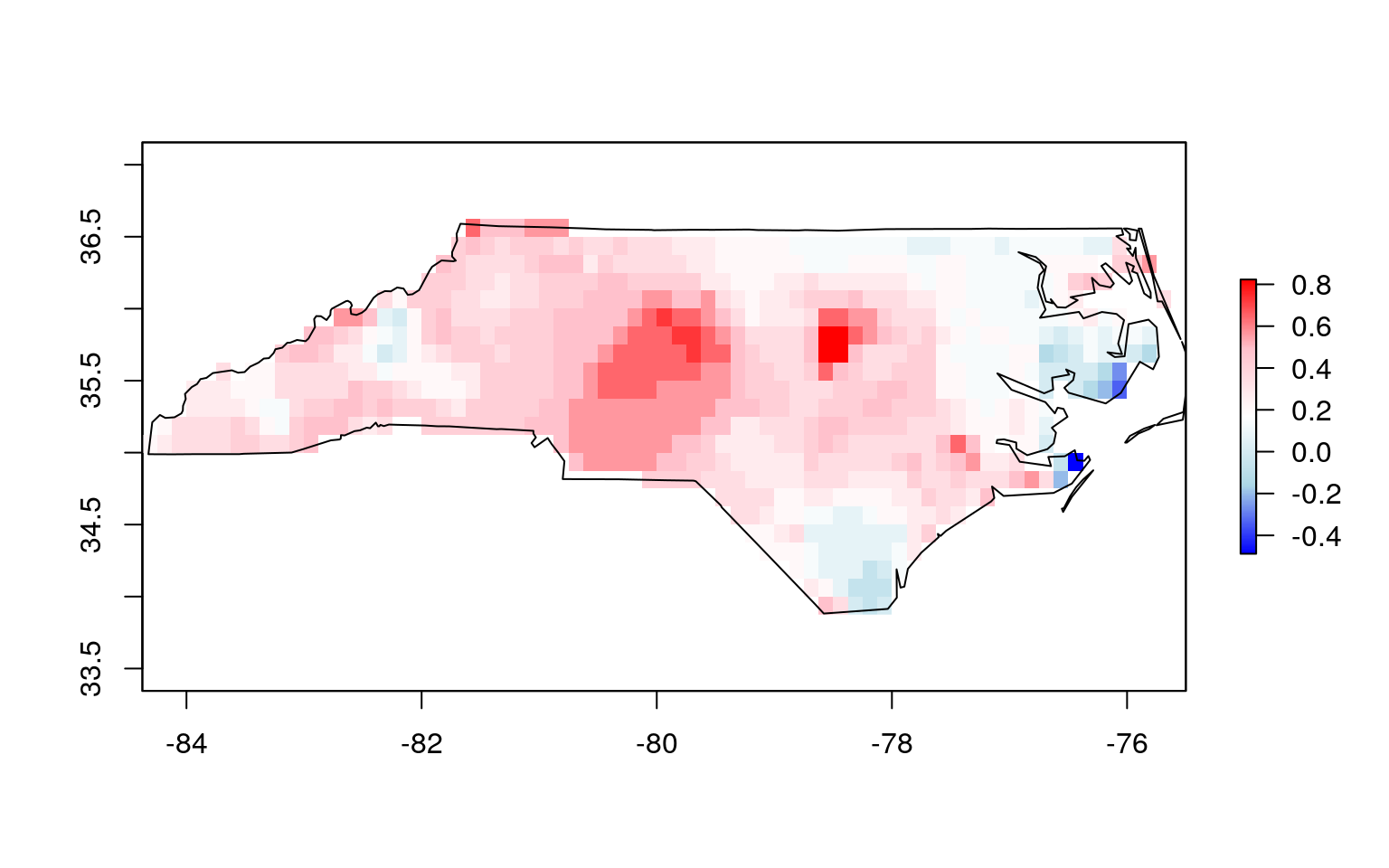
masked_eddi <- mask(cropped_eddi, roi_sp)You can plot the masked EDDI raster along with the ROI to confirm: